If you have any experience with machine learning or its sub-discipline of deep learning, you probably know that we usually use gradient descent and its variants in the process of training our models and neural networks. In the early days, and you might have caught a glimpse of that if you ever did Andrew Ng’s MOOC or went through Michael Nielsen’s book Neural Networks and Deep Learning, we used to code the gradients of the models by hand. However, as the models got more complex this became more cumbersome and tedious! This is where the modern computation libraries like pyTorch, Tensorflow, CNTK, Theano and others shine! These libraries allow us to just write our math and they automatically provide us with the gradients we want, which allowed the rapid deployment of more and more complex architectures. These libraries are able to “automagically” obtain the gradient via a technique called Automatic Differentiation. This intro is to demystify the technique of its “magic”!
This introduction will be covered in two parts, this part will introduce the forward mode of automatic differentiation, and next one will cover the reverse mode, which is mainly used by the deep learning libraries like pyTorch and TensorFlow. By the end of this post, we’ll be able to train a simple linear regression model using gradient descent without explicitly writing the a function to compute the loss’s gradient! Instead, we’ll let forward mode automatic differentiation do it for us.
These posts are not a tutorial on how to build a production ready computational library, there so much detail and pitfalls that goes into that, some of which I’m sure I’m not even aware of! The main purpose of this post is to introduce the idea of automatic differentiation and to get a grounded feeling of how it works. For this reason and because it has a wider popularity among practitioners than other languages, we’re going to be using python as our programming language instead of a more efficient languages for the task like C or C++. All the code we’ll encounter through the post resides in this GitHub repository.
A Tale of Two Methods
One of the most traditional ways to compute the derivative of a function, taught in almost all numerical computations courses, is the via the definition of the derivate itself:
\[f'(x) = \lim_{h \rightarrow 0} \frac{f(x + h) - f(x)}{h}\]However, because we can’t divide by zero without the computer rightfully yelling at us, we settle to having $h$ to be a very small value that is close to but not zero. We truncate the zero to an approximate value and this results in an error in the derivative’s value that we call the truncation error. Dealing with real numbers inside a digital computer almost always suffers from an error and loss in precision due to the fact that the limited binary representation of the number in memory cannot accommodate for the exact real value of the number, so the number gets rounded off after some point to be stored in a binary format. We call such error a roundoff error.
Even with the roundoff error, the truncation error in the derivative calculation is not that big of a deal if our sole purpose is to just compute the derivative, but that’s rarely the case! Usually we want to compute a derivative to use it in other operations, like in machine learning when the derivative is used to update the values of our model’s weights, in this case the existence of an error becomes a concern. When the it starts to propagate through other operations that suffer their own truncation and roundoff errors, the original error starts to expand and results in the final operation being thrown off its exact value. This phenomenon is called error propagation and its one of the major problem that face such a way to compute derivatives. It’s possible to reformulate the limit rule a bit to result in less truncation error, but with every decrease in error we make we get an increase in the computational complexity needed to carry out the operation.
One other approach to compute the derivative of a function is by exploiting the fact that taking the derivative of a function is a purely mechanical process. Let’s for example examine how we can take the derivative of the function:
\[f(x)=\left(\sin x\right)^{\sin x}\]We can compute that derivative, a step-by-step, using the elementary rules of differentiation as follows:
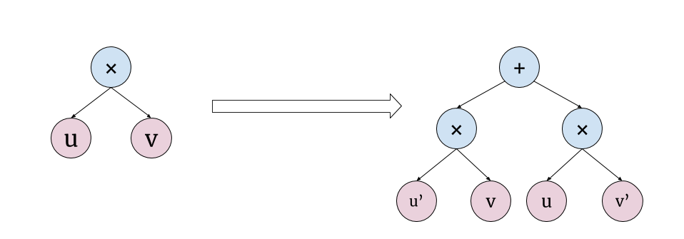
\[\begin{split} f'(x) & = \left(\left(\sin x\right)^{\sin x}\right)' = \left(e^{\sin x \ln \sin x}\right)' = \left(e^{u(x)}\right)' \\ & = \frac{df}{du}\times\frac{du}{dx} = \frac{d}{du}\left(e^{u}\right) \times \frac{d}{dx}\left(\sin x \ln \sin x\right)& \text{(Chain Rule)} \\ & = e^u \frac{d}{dx}\left(\sin x \ln \sin x\right) & \text{($e^x$ Rule)} \\ & = e^u\left(\frac{d}{dx}\left(\ln \sin x\right) \sin x + \frac{d}{dx}\left(\sin x\right) \ln \sin x\right) & \text{(Product Rule)} \\ & = e^u\left(\frac{d}{dx}\left(\ln v(x)\right) \sin x + \cos x \ln \sin x\right) & \text{($\sin$ Rule)} \\ & = e^u\left(\left(\frac{d}{dv}\left(\ln v\right) \times \frac{d}{dx}(\sin x)\right) \sin x + \cos x \ln \sin x\right) & \text{(Chain Rule)} \\ & = e^u\left(\left(\frac{1}{v}\frac{d}{dx}(\sin x)\right) \sin x + \cos x \ln \sin x\right) & \text{($\ln$ Rule)} \\ & = e^u\left(\frac{\cos x}{v} \times \sin x + \cos x \ln \sin x\right) & \text{($\sin$ Rule)} \\ & = \left(\sin x\right)^{\sin x}\left(\frac{\cos x}{\sin x} \times \sin x + \cos x \ln \sin x\right) & \text{(Substitution)}\\ & \color{red} = \left(\sin x\right)^{\sin x}\left(\cos x + \cos x \ln \sin x\right) \\ & \color{red} = \left(\sin x\right)^{\sin x}\cos x\left(1 + \ln \sin x\right) \end{split}\]By observing the step-by-step solution, it appears how mechanical the differentiation process is and how it can be represented as an iterative application of a few simple rules. An approach to implement this is to construct some sort of an abstract syntax tree (AST) of the given expressions, this tree is then traversed and each node gets transformed using the simple rules to another AST node representing the derivative of that node. The following figure shows this process for single multiplication node.
This method of computing the derivative is called symbolic differentiation as it manipulates the symbols of the expressions directly to arrive at the derivative. This method overcomes the error problem in our earlier method, because the final expression of the derivative will only suffer from the computer’s roundoff error but there will be no truncation error; the value of the derivative will be as exact as it can be represented in a digital computer. As nice as this is, the symbolic differentiation suffers from two drawbacks.
Go back and take a look on the step-by-step solution of the derivative, notice the two red steps in the end? These steps are not immediately reachable by symbolic differentiation engine! Such engine would usually stop at the last black step without the simplification of the expression. It’s obvious that evaluating the unsimplified expression is not as efficient as evaluating the simplified one; there are redundant (like the $\cos x$ in the two terms within the parentheses) and useless computations (like $\frac{1}{\sin x}\sin x$ in the first term between the parentheses) involved! This problem becomes more serious when the expression to differentiate becomes more complex and redundant and useless computations keep popping up all over the derivative. Implementing an optimizer that would simplify the derivative expression is not impossible, but it will introduce extra complexity in both the maintenance of such implementation and the computational cost.
Another drawback to the symbolic approach is that it doesn’t lend itself nicely to programmatic constructs. Say that you created a function transform(x) that takes a vector of values and applies a series of calculations that involves control branches and loops to transform that vector into a single value. It’s not really clear how to calculate the derivative of such transform using symbolic differentiation as it is clear with our earlier numerical approach. This kind of painful Trade-off between the two methods is one of the main motivators behind the adoption of the method that we’ll start to investigative now, which is automatic differentiation (AD).
Dual Numbers
Let’s take a close look at the Taylor series of any function $f(x)$ around the point $x=a$:
\[f(x) = \sum_{k=0}^{\infty}\frac{f^{(k)}(a)}{k!}(x-a)^k = f(a) + f'(a)(x-a) + \sum_{k=2}^{\infty}\frac{f^{(k)}(a)}{k!}(x-a)^k\]wouldn’t it be nice if we could plug in some value of $x$ that would preserve us the term containing $f’(a)$ and make the rest of the infinite sum evaluate to exactly zero? In that way there would be not truncation error and we could get the value of the derivative by just evaluating the function itself! Unfortunately, it’s easy to see that there’s no real value that would achieve us that. The only two ways the infinite sum would evaluate to exactly zero would be either if all the higher-order derivatives $f^{(k)}(a)$ are zeros; in which case the method would not be general to all possible functions (it will actually be limited to only linear functions), or $(x-a)^k$ is zero which means that $x=a$; in which case the term including $f’(a)$ would also evaluate to zero and we lose the first derivative.
However, having no real solutions to a problem doesn’t usually stop the mathematicians from finding a solution outside the real realm, and just as they constructed the set of complex numbers to account for the value of $\sqrt{-1}$, we can devise our own set of numbers to achieve our goal! We’ll define this new set as the set of all numbers in the form $a + b\epsilon$ where $a,b \in \mathbb{R}$ and $\epsilon \neq 0$ while $\epsilon^2=0$ This cannot be satisfied with a single number like $\sqrt{-1}$ does for $i$, $\epsilon$ is a matrix whose square has all elements as zeros, something like $\epsilon = \binom{0 \hspace{1em} 1}{0 \hspace{1em} 0}$ for which $\epsilon^2 = \binom{0 \hspace{1em} 0}{0 \hspace{1em} 0}$. These matrices are called nilpotent which means “without power”.. We’ll call this new set the set of Dual Numbers and we’ll denote $a$ as the real component and $b$ as the dual component. Now let’s plug in $x = a + b\epsilon$ into our Taylor series and see what happens:
\[\begin{split} f(a + b\epsilon) & = f(a) + f'(a)b\epsilon + \sum_{k=2}^{\infty}\frac{f^{(k)}(a)}{k!}b^k\epsilon^k \\ & = f(a) + f'(a)b\epsilon + \underbrace{\epsilon^2\sum_{k=2}^{\infty}\frac{f^{(k)}(a)}{k!}b^k\epsilon^{k-2}}_{0} \\ & = f(a) + f'(a)b\epsilon \end{split}\]If we went ahead and set $b = 1$, we get that $f(a + \epsilon) = f(a) + f’(a)\epsilon$; which means that evaluating a function using dual number with a real component $a$ and dual component $1$ results in another dual number that has the value of $f(a)$ as its real component and “automatically” its derivative at $a$ as the dual component, no symbol manipulations, and no truncation errors! And if we generalized that to say that a dual number represents some value and its derivative, we can think of the representation of $x=a+b\epsilon$ as $a$ being the value of $x$ and $b$ as its derivative with respect to itself, which makes $b = 1$ as we set it earlier.
Operations on Dual Numbers
Like any other number system, we can define a set of operations on its members. Like addition and multiplication for example:
\[(a + b\epsilon) + (c + d\epsilon) = (a + c) + (b + d)\epsilon\] \[(a + b\epsilon)(c + d\epsilon) = ac + ad\epsilon + bc\epsilon + bd\epsilon^2 = ac + (bc + ad)\epsilon\]The cool thing about those operations is that if we used them with the fact that for any function $f(x + \epsilon) = f(x) + f’(x)\epsilon$ we’ll find that these operation “automatically” provide us with the simple rules of differentiation we’re already familiar with! E.g. with the two rules of addition and multiplication we just derived we can get:
\[\begin{split} f(x + \epsilon) + g(x + \epsilon) & = \left[f(x) + f'(x)\epsilon\right] + \left[g(x) + g'(x)\epsilon\right] \\ & = \left[f(x) + g(x)\right] + \left[f'(x) + g'(x)\right]\epsilon \end{split}\] \[\begin{split} f(x + \epsilon)g(x + \epsilon) & = \left[f(x) + f'(x)\epsilon\right]\left[g(x) + g'(x)\epsilon\right] \\ & = \left[f(x)g(x)\right] + \left[f'(x)g(x) + f(x)g'(x)\right]\epsilon \end{split}\]Which reflect the addition and product rules of differentiation respectively! We could also derive more complex operations on dual numbers using the same fact that $f(a + b\epsilon) = f(a) + f’(a)b\epsilon$, for example:
\[\sin(a + b\epsilon) = \sin a + (\sin a)'b\epsilon = \sin a + (\cos a)b\epsilon\] \[\ln(a + b\epsilon) = \ln a + (\ln a)'b\epsilon = \ln a + \frac{b}{a}\epsilon\]The fact that we can derive such operations and that these operations “automatically” contain the necessary rules for differentiation makes the system of dual numbers the ideal candidate to build the first mode of automatic differentiation, which is called the Forward Mode.
AD: Forward Mode
The first thing we need to make in order to implement the forward mode of AD is start by implementing the dual numbers themselves. We can simply implement them via a class that contains two real attributes, one for the real component and the other for the dual component.
class DualNumber:

    def __init__(self, real, dual):

        self.real = real
        self.dual = dual
The important thing to do is to allow objects of this class to behave correctly with arithmetic operations in the way we just specified in the previous section. Such thing can be achieved with something known in programming languages as Operator Overloading. With operator overloading, a programming language allows us to change the functionality of pre-defined operators (such as +, -, *, ** in python) according the type of arguments the operation takes, so say a + operator works in the ordinary way with ordinary real numbers while working in a different way with a user-defined type like that DualNumber class we just created.
In python, arithmetic operator overloading is done for some arbitrary class via implementing some special named methods reserved for numeric type emulation. For example, to overload the + operator, we need to implement a method called __add__(self, other) that takes our dual number object itself as an operand and another object for the other operand.
from numbers import Number

class DualNumber:

    def __init__(self, real, dual): ...

    def __add__(self, other):
        if isinstance(other, DualNumber):
            return DualNumber(self.real + other.real, self.dual + other.dual)
        elif isinstance(other, Number):
            return DualNumber(self.real + other, self.dual)
        else:
            raise TypeError("Unsupported Type for __add__")
The way this works is very simple: we first check if the other operand is another dual number, if it is we return a new one with the sum of the real components and the sum of the dual components. If the other operator was just a real number, we return a new object with the same dual component and the real component with the new real operand added to it! If it’s neither we just throw an error saying that this operand type is not supported. That way we could perform addition operations between dual numbers and themselves, and between dual numbers and real ones, at least when the real numbers comes on the right!
x = DualNumber(4, 7)
y = DualNumber(-1, 5)

z = x + y  # valid operation: returns a DualNumber(3, 12)
w = x + 10 # valid operation: returns a DualNumber(14, 7)

v = 4 + y  # throws a TypeError
What’s the problem was the last operation then? why does it break when the real number comes on the left of the operator?!
This has to do with the way python calls for the operator implementation. By default, the implementation of the operand to the left is the one called for the operator; and the left operand here has no idea how to deal with our DualNumber class! Python however provides a way around this: if the operand on the left has no idea how to operate on with the one on the right, the right one’s implementation of a another special function called __radd__(self,other) is called instead (r for reverse). So in order to allow for addition operations where the real operand can come on the left, we need to implement that method into our class.
from numbers import Number

class DualNumber:

    def __init__(self, real, dual): ...

    def __add__(self, other): ...

    def __radd__(self, other):
        # this time we know that other is a real and cannot be DualNumber
        return DualNumber(self.real + other, self.dual)
You can see that this case is already included in the code we wrote for the regular __add__ method, so in accordance to the DRY principle (Don’t Repeat Yourself), we create a separate function that is capable of carrying out both modes of operation and make each of the special functions call that. This is particularly useful when the code for each of the modes tend to be big and using that abstraction cuts the amount of code in half (like in the overloading of the division operation). So our implementation for the addition operation would look like that:
from numbers import Number

class DualNumber:

    def __init__(self, real, dual): ...

    def _add(self, other):
        if isinstance(other, DualNumber):
            return DualNumber(self.real + other.real, self.dual + other.dual)
        elif isinstance(other, Number):
            return DualNumber(self.real + other, self.dual)
        else:
            raise TypeError("Unsupported Type for __add__")

    def __add__(self, other):
        return self._add(other)

    def __radd__(self, other):
        return self._add(other)
However, a little caution needs to be taken when the operator is not commutative, like subtraction, division and power. In such case we need an additional flag that tells us if the dual number is coming first or not so that we could set that flag off in the reverse operation. Here’s how the subtraction operation would look with such a flag.
from numbers import Number

class DualNumber:

    ...

    def _sub(self, other, self_first=True):
        if self_first and isinstance(other, DualNumber):
            return DualNumber(self.real - other.real, self.dual - other.dual)
        elif self_first and isinstance(other, Number):
            return DualNumber(self.real - other, self.dual)
        elif not self_first and isinstance(other, Number):
            return DualNumber(other - self.real, -1 * self.dual)
        else:
            raise TypeError("Unsupported Type for __sub__")

    def __sub__(self, other):
        return self._sub(other)

    def __rsub__(self, other):
        return self._sub(other, self_first=False)
The rest of the class implementation which also includes multiplication, division and powers, can be found in the code repository in the dualnumbers.py file. It’s fully commented and it follows exactly the same pattern of coding we used in the two operations here, the difference is in the math of each operation. The full derivation of these different math of can be found in Dual-Algebra.pdf file, also in the repository.
The next step after we defined what a dual number is and how it behaves is to create some mathematical functions that can handle the dual numbers. These can be easily defined as directly implementing similar math like those we got earlier for the $\sin$ and $\ln$ functions using the python’s real math library math. An implementation for the $\sin$ function would go like this:
from dualnumbers import DualNumber
import math as rmath

def sin(x):
    if isinstance(x, DualNumber):
        return DualNumber(rmath.sin(x.real), rmath.cos(x.real) * x.dual)
    else:
        return rmath.sin(x)
It simply checks if the argument is dual, if it is then it returns the dual evaluation of the function. Otherwise it just falls back on the real function. This would allow us to use these functions interchangeably between dual and real numbers. dmath.py file contains this method alongside a few other methods for different mathematical functions, the follow the same pattern as the sin method we just implemented and their specific math can also be found in the Dual-Algebra.pdf file. Both dmath.py and dualnumbers.py are contained in a package called dualnumbers and the repository contains a Dual-Math notebook that showcases the different operations implemented in that package.
We’re now ready to implement our forward mode of AD: all we need to do is take a function and the value of its variable at which we want to calculate the derivative, we then wrap this value into a dual number with a dual component of 1 and pass it to the function. The dual component of the resulting number is the derivative we want!
from dualnumbers import DualNumber

def derivative(fx, x):
    return fx(DualNumber(x, 1)).dual
We implement this method into a module called forward within a package we’ll call autodiff. Let’s see how this works with the function we differentiated earlier: $f(x) = (\sin x)^{\sin x}$. At $x = \frac{\pi}{4}$ we can calculate the derivative from the resulting expression and find that it’s $0.3616192241$, we’ll also find that our derivative function returns the same value:
from autodiff.forward import derivative
from math import pi
import dualnumbers.dmath as dmath


fx = lambda x: dmath.sin(x) ** dmath.sin(x)

print("{:.10f}".format(derivative(fx, 0, [pi/4])))  # prints 0.3616192241
However, we’re not going to have the derivative’s expression every time to check it’s value against the our derivative method, actually the point of having an AD system is to elevate the need to do derivations by hand! Instead, to ensure the correctness of our derivatives, we resort to a technique known in the Machine Learning field as gradient checking. In this technique we essentially compare the derivate from AD to a numerical derivate calculated using the limit method we saw first thing here. The limit method gives us an approximate value that we’re sure of its correctness (because it is the definition of the derivative), so the value of our AD method should be close to the numerical one within an acceptable error defined by both absolute and relative errors.
def check_derivative(fx, x, suspect):
    h = 1.e-7
    rerr = 1.e-5
    aerr = 1.e-8

    numerical_derivative = (fx(x + h) - fx(x)) / h
    accept_error = aerr + abs(numerical_derivative) * rerr

    return abs(suspect - numerical_derivative) <= accept_error
We can test that with a new function like $f(x) = x^22^x$ that we don’t know its derivative at $x=\frac{1}{2}$ beforehand:
from autodiff.forward import derivative, check_derivative

fx = lambda x: (x ** 2) * (2 ** x)

ad_derivative = derivative(fx, 0.5)

print("{:.10f}".format(ad_derivative))  # prints 1.6592780982
print("{}".format(check_derivative(fx, 0, [0.5], ad_derivative)))  # prints True
How about functions with multiple variables then? How can we compute the partial derivative with respect to each variable?
Remember that we treated the dual component of the variable as the variable’s derivative with respect to the differentiation variable, which in the single variable case was itself and that made its dual component be set to 1. We can extended the same rational to include multiple variables; to get the partial derivative of a function with respect to a certain variable, we set that variable’s dual component to 1 and all the other variables should have a dual component of 0 that represents their derivatives with respect to that variable. We can encourage that method by looking at the math of the simplest multi-variables function, the two variables function The math for a more general argument can be a little tedious to work with, that’s why we suffice with the two variables case. However, a general argument could be made using Taylor’s series generalization in multiple variables.. For a function $f(x,y)$ evaluated with dual numbers $a+b\epsilon, c+d\epsilon$ for $x,y$ respectively, its Taylor series has the form:
\[f(a+b\epsilon, c+d\epsilon)= f(a, c) + \left(\frac{\partial f(a, c)}{\partial x}b + \frac{\partial f(a, c)}{\partial y}d\right)\epsilon\]If we’d like to get the derivative with respect to $x$ we just set its dual component to 1 and $y$’s dual component to 0 as we just discussed, that would get us a dual number with just the partial derivative with respect to $x$ as its dual component:
\[f(a+\epsilon, c+0.\epsilon)= f(a, c) + \frac{\partial f(a, c)}{\partial x}\epsilon\]The other way around would get us the partial derivative with respect to $y$. With that we can implement a more general version of our derivative method that could work with any function of any number of variables, we just specify the which variable we want to differentiate with respect to and we provide the list of variables’ values instead of a single value.
def derivative(fx, wrt, args):

    dual_args = []
    for i, arg in enumerate(args):
        if i == wrt:
            dual_args.append(DualNumber(arg, 1))
        else:
            dual_args.append(DualNumber(arg, 0))

    return fx(*dual_args).dual
Here wrt is the zero-based index of the variable we’d like to differentiate with respect to as it appears in arguments of the function fx, and args is a list of values representing the point we want to know the derivative at.
We can also generalize our check_derivative in the same way by adding $h$ only to the value of the variable we’re differentiate with respect to.
def check_derivative(fx, wrt, args, suspect):
    h = 1.e-7
    rerr = 1.e-5
    aerr = 1.e-8

    shifted_args = args[:]
    shifted_args[wrt] += h

    numerical_derivative = (fx(*shifted_args) - fx(*args)) / h
    accept_error = aerr + abs(numerical_derivative) * rerr

    return abs(suspect - numerical_derivative) <= accept_error
For example, let’s see how that would work with a function like:
\[f(x,y,z) = \sin(x^{y + z}) - 3z\ln x^2y^3\]we’d like the partial derivative with respect to $y$ at $(0.5, 4, -2.3)$:
from autodiff.forward import derivative, check_derivative
import dualnumbers.dmath as dmath


f = lambda x,y,z: dmath.sin(x ** (y + z)) - 3 * z * dmath.log((x ** 2) * (y ** 3))
ad_derivative = derivative(f, 1, [0.5, 4, -2.3])

print("{:.10f}".format(ad_derivative))  # prints 4.9716845517
print("{}".format(check_derivative(f, 1, [0.5, 4, -2.3], ad_derivative)))  # prints True
Back now to the original purpose we started this post with, which is computing gradients. The gradient of a function $f(\mathbf{x})$ where $\mathbf{x}$ is a vector of $n$ variables is the vector:
\[\nabla f = \begin{bmatrix}\frac{\partial f}{\partial x_1} & \dots & \frac{\partial f}{\partial x_n}\end{bmatrix}\]We can easily compute that by calling our derivative function $n$ times on the function, each time with a different value for the wrt argument.
def gradient(fx, args):

    grad = []
    for i,_ in enumerate(args):
        grad.append(derivative(fx, i, args))

    return grad
We could try this gradient method out using a simple linear regression model that we’ll train using gradient descent. We’ll be using a synthetic dataset of 500 points generated randomly from a noisy target $y = 1.4x - 0.7$. We’ll use the mean-squared error as our loss measure in estimating the slope $\theta_1$ and the intercept $\theta_0$:
and with a learning rate of $\alpha$, our iterative gradient-based update rules would be:
\[\theta_i = \theta_i - \alpha\frac{\partial}{\partial \theta_i}J(\theta_0, \theta_1)\]import random
from autodiff.forward import gradient
target = lambda x: 1.4 * x - 0.7 # synthizing model
# generating a synthetic dataset of 500 datapoints
Xs = [random.uniform(0, 1) for _ in range(500)]
ys = [target(x) + random.uniform(-1, 1) for x in Xs] # target + noise
def loss(slope, intercept, alpha):
loss_value = 0
for i in range(500):
loss_value += (ys[i] - (slope * Xs[i] + intercept)) ** 2
return 0.002 * loss_value
# initial values of training parameters
slope = 0.1
intercept = 0
learning_rate = 0.1
# training loop
for _ in range(10000):
grad = gradient(loss, [slope, intercept, 1])
# update the parameters using gradient info
slope -= learning_rate * grad[0]
intercept -= learning_rate * grad[1]
# print the final values of the parameters
print("Slope {:.2f}".format(slope)) # prints "Slope 1.44"
print("Intercept {:.2f}".format(intercept)) # prints "Intercept -0.73"
By running this script (which can be found with all the previous ones in the Forward-AD notebook in the repository), we can see that the final estimations are pretty good! Moreover, we were able to see how our forward AD methods works seamlessly with a programmatic construct like the loss function that involves control flow operations like loops, in an exact way with no truncation errors or inefficient symbol manipulations. However, calculating gradients with forward AD has an inefficiency of its own!
For a function $f(\mathbf{x})$ where $\mathbf{x}$ is a vector of $n$ variables; if the function itself has a computational complexity $O(K)$, then the gradient would have a complexity of $O(nK)$ which is not that of a trouble when $n$ is small. However, for something like a neural network where there could be hundreds of millions of parameters, hence $n$ is in the order of hundreds of millions, we’ll be in big trouble! We need another AD method that could handle such a large numbers of parameters more efficiently, and that’s what we’re going to do in the next part!
In part-2, we’ll cover reverse mode AD and build our own mini deep learning library and use it to train a neural network on MNIST dataset! Stay tuned.

Comments