In the previous part of this series, we learned about forward mode automatic differentiation, and we saw its limitations when we need to calculate the gradient of a function of many variables. Today, we’ll into another mode of automatic differentiation that helps overcome this limitation; that mode is reverse mode automatic differentiation. This mode of AD is the one used by all major deep learning frameworks like Tensorflow, Pytorch, MinPy, Jax, Chainer and others.

In this part of the series, we’ll learn together how reverse AD works and well make our learnings concrete by getting our hands dirty and building a mini deep learning framework of our own and train a small neural network with it. While we’re not expected to implement deep learning frameworks on our own in, doing so here would give us a much deeper understanding of how the existing frameworks operate and much deeper appreciation for the mathematical and engineering efforts that has been put into these frameworks.

I’m not going to lie to you, this journey is a bit long. But trust me, it’ll be very rewarding when you successfully train your neural network using a framework that you have built with your own hands. However, to make pausing and breaking possible, I have structured the article into sections that you could read separately through consecutive settings. Here’s a summary of what we’ll work on in each section:

• Starting from the End in which we’ll learn the mathematical basis of reverse mode AD and visualize it in action
• Implementing Reverse Mode AD
  • Building a Computational Graph where we’ll start with the fundamental building block to implement reverse AD by creating a computational graphs framework built on numpy.
  • Computing Gradients is the part where we learn how to the compute the derivatives of functions involving two types of multi-dimensional array operations:
    • Reduction Operations like np.mean and np.max
    • Arithmetic Operations like adding two arrays and carrying out the dot product
    • Unbroadcasting Adjoints where we learn to match derivatives with their variables shapes even if numpy has performed some broadcasting.
  • Putting Everything Into Action is where we put all the puzzle pieces together to get a functioning deep learning framework that we could use for:
    • Training a Neural Network while
    • Avoiding Numerical Instability

All the code that is written/mentioned throughout this post, along with the scripts and examples, all can be found in this GitHub repository. I’d really appreciate if you could mention and error that you come across or enhancements you have on the writing or the code. All contributions are welcome. You can create an issue/PR on the project repository and the blog repository as well, or you can reach out to me directly if you’d like.

Now, let’s jump in!

Starting from the End

Let’s consider a function like $f(x) = \sin(2\ln x)$. Assume that all the calculators in the world disappeared in bizarre accident and we need to evaluate this function by hand! To evaluate it correctly we need to go through the following order of evaluation:

Another way to look at this evaluation order is by decomposing the expression to simpler sequential calculations; so we could say that $w_0=\ln x$, $w_1=2w_0$, and finally $f = \sin w_1$. Using this decomposition we want to calculate the derivative $\frac{\partial f}{\partial x}$ when $x=2$ (we’ll use the partial symbol $\partial$ for all derivatives from now on). Let’s first go forward from start to finish and evaluate the values of the intermediate steps up to the value of $f$:

In our decomposition, we have $f$ as a function of $w_1$, so we start by calculating $\frac{\partial f}{\partial w_1}$ which equals to $\cos w_1 \approx 0.183$. We then have $w_1$ as a function of $w_0$, which makes $f$ implicitly a function of $w_0$ as well. Using the chain rule we can write:

We already know $\frac{\partial f}{\partial w_1}$ form the previous step, and we can easily get $\frac{\partial w_1}{\partial w_0}$ from the definition of $w_1$, which is just $2$, giving us $\frac{\partial f}{\partial w_0}\approx 2\times0.183 \approx 0.366$. Taking this derivative and going one last step back to $w_0$, which is a direct function of $x$, we can write by also using the chain rule:

A better way to look at this process is visually. Instead of writing down the intermediate steps like that, we visualize the whole operation as a computational graph, a direct graph where the nodes represent variables, constants or simple binary/urinary operations; and the edges represent the flow of the the values from each node to the other. Our function at question here can be represented by the following computational graph:

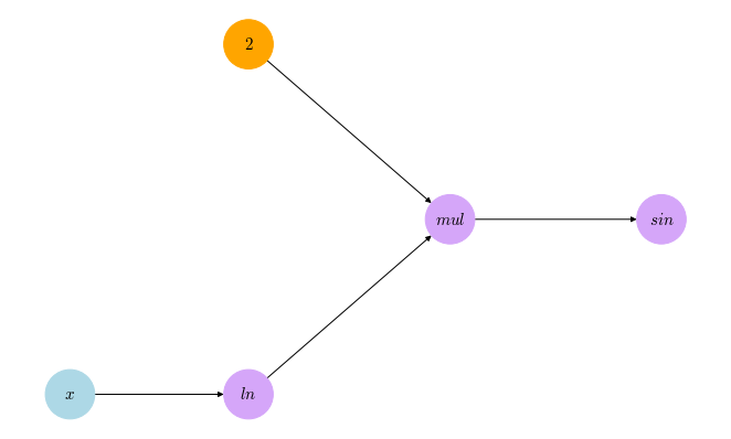
Throughout the rest of the post, all the computational graphs we’ll see will follow the same color code: lightblue for variables, orange for constants, and purple for operations. We can see that this computational graph corresponds to the decomposition we made earlier, with the ‘ln’ node representing $w_0$, ‘mul’ node for $w_1$, and ‘sin’ node for $f$. Using the tool of computational graph, we can more visually see the process of propagating the derivative backward and applying the chain rule in th following animation:

With this step-by-step animation, we can see how by traversing the computational graph in a breadth-first manner starting from the node representing our final function, we can propagate the derivatives backwards until we reach the desired derivative. At each step, the current operation node (the one highlighted in green) propagates $f$’s derivative with respect to itself (the number written on the highlighted edge) to one of its operands nodes (the one at the other end of that highlighted edge); using the chain rule, $f$’s derivative w.r.t. the current operand node is evaluated and will be used in the next steps.

So, following the path down the computational graph till we reach our variable gives us the derivative with respect to that variable. However, the examples we saw had only one path leading to the variable $x$, how about a function like $f(x) = x^2 + 2^x$? Let’s see how the computational graph for this function looks like:

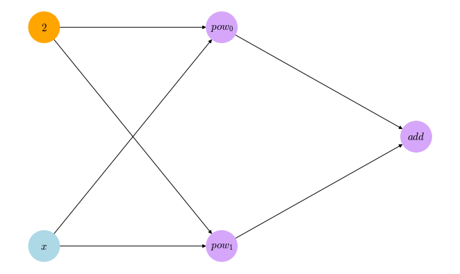
In such function, we have the variable $x$ contributing to two computational paths, so it will receive two derivatives when we start propagating the derivatives backwards, which poses a question about how the final derivative with respect to $x$ would look like! Maybe we can add the derivatives from the two paths to get the final one? While this sounds as just an answer based on simple intuition, it is actually the correct one! The rigorous base for this answer is what’s called the multivariable chain rule Here’s a very nice introduction on the multivariable chain rule from KhanAcademy. In it’s simplest form, which is the form we’re concerned with here, the rule says that for a function $f$ that is a function of two other functions of $x$, that is $f = f(g(x), h(x))$, the derivative of $f$ with respect to $x$ is:

By applying this idea to the backward propagation of derivatives in the computational graph of $x^2 + 2^x$ at $x=4$, we can see how the value of $\frac{\partial f}{\partial x}$ gets accumulated on as new propagated derivatives arrive at it:

This justifies why we initially set the derivatives at the variables (and at each other node) to zero. It also explains why we traverse the graph breadth-first; we want to make sure that all the contributions to a node’s $f$ derivative (in AD lingo, this derivative is called the adjoint) has arrived before taking its value and propagating it further back through the graph.

A very important question you might have by this point is: why bother? Whats the point of going at the derivative from the other way around and keeping up with all that hassle?! The answer to this question becomes clear when we look at the same process applied to a multivariable function; for example, $f(x,y,z) = \sin(x+y) + (xy)^{z}$ at $(x,y,z) = (1, 2, 3)$.

See what happened here? We were able to get the derivative with respect to all three variables in just a single run through the graph! So, if we have a function of $n$ variables that takes $O(K)$ time to traverse it’s computational graph, it will take $O(K)$ time to obtain all the $n$ derivatives, no matter how big $n$ is! This is why we bother with going at the derivative from the end and backwards! This method gives us a mechanical way to automatically obtain the derivatives of a multivariable function without having to suffer the performance hit that forward mode AD had. This approach to differentiation is what constitutes the second mode of AD that we’ll see now, the reverse mode.

Implementing Reverse Mode AD

Building a Computational Graph

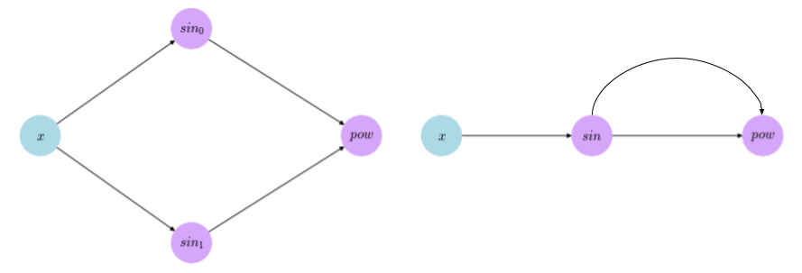
The first thing we need to create in order to implement the reverse mode of AD is to create a way that would allow us to build computational graphs that represent the computations we express. There are two design choices when we go about implementing computational graphs; the first is to initially build the graph then run the necessary computations by feeding values to that graph, the other is to build a computational graph representation along with carrying out the calculations. The first choice, which is commonly referred to as static computational graphs, is what frameworks like TensorFlow and Torch use. The advantage of this choice is the ability to optimize the graph before running the calculations; big computational graphs usually could benefit from some optimizations that would allow the computations to be run faster and allow a more efficient usage of resources. A simple example of that could be found in the function $f(x) = (\sin x)^{\sin x}$; an optimizer on a static graph can turn it form the one on the left to the one on the right, with one less computation to worry about.

However, statically built graph are kind of hard to debug, and doesn’t not play nicely with regular programming constructs like conditional branches and looping. On the other hand, the second choice builds the graph dynamically along with carrying the computations. Many frameworks; like PyTorch, MinPy, and Chainer; adapted this choice as it allows for a workflow that is much easier to understand and to debug, but it loses the ability to optimize the computations. Even Tensorflow, which started with static graphs, now supports the building the graphs dynamically. The choice between the two is a trade-off between efficiency and simplicity, and because the goal here is to provide a simple introduction to the topic, we’ll go with dynamic graphs as our design choice.

We are going to be using numpy as our base computational engine off which we’ll build the computational graphing tool. The essential element of a graph is a node; we can represent each node as an object and the edges could be specified by attributes in the node object pointing to other nodes. Because we want our nodes to be indifferent from regular numerical values, we’ll start be defining a base Node class that extends numpy’s essential data structure, the ndarray. In that way, we can get our nodes to behave exactly the same as ndarrays while having the ability to add the necessary extra functionalities we need to create the graphs. We follow numpy’s official guide on extending the ndarray object.

class Node(np.ndarray):

    def __new__(subtype, shape,
                dtype=float,
                buffer=None,
                offset=0,
                strides=None,
                order=None):

        newobj = np.ndarray.__new__(
            subtype, shape, dtype,
            buffer, offset, strides,
            order
        )

        return newobj

from this object we extend three other classes that represent the three types of nodes we saw in the earlier graphs; an OperationalNode, a ConstantNode and a VariableNode. These extensions are fairly simple and only has one addition to the base Node class, which is a static method called create_using. This method allows us to create nodes on the fly using a numpy’s ndarray or a number without needing to pass the arguments of the base’s __new__ method separately, we let this method take care of that and also add any necessary extra attributes to the object. We can first see this in action with the VariableNode class in which the create_using method takes a number or an ndarray value along with an optional name and returns an VariableNode object initialized at that value with a name attribute pointing to the name given or an auto-generated name if none is given.

class VariableNode(Node):

     # a static attribute to count the unnamed instances
     count = 0

     @staticmethod
     def create_using(val, name=None):

        if not isinstance(val, np.ndarray):
            val = np.array(val, dtype=float)

        obj = VariableNode(
            strides=val.strides,
            shape=val.shape,
            dtype=val.dtype,
            buffer=val
        )
        if name is not None:
            obj.name = name
        else:
            obj.name = "var_%d" % (VariableNode.count)
            VariableNode.count += 1

        return obj

The ConstantNode class looks exactly like the VariableNode class except for the fact that we use “const_“ instead of “var_“ in the auto generation of the node’s name; we created separate classes for them just to be able to distinguish between them in runtime, but in practice the ConstantNode would need more additions, like for example, some overloads for the +=, -=, *=, and /= operators to prevent the modification of the constant’s initialized value, but we’re dropping that here.

The last type of nodes is the OperationalNode class. We want an operational node to know which operation it reflects (addition, subtraction, multiplication, … etc), what is the result value of that operation, what are the operands nodes, and to have a name just like the other nodes have. Because of these requirements,the create_using method of the operational node looks a bit different than in the others.

class OperationalNode(Node):

    # a static attribute to count for unnamed nodes
    nodes_counter = {}

    @staticmethod
    def create_using(opresult, opname, operand_a, operand_b=None, name=None):

        obj = OperationalNode(
            strides=opresult.strides,
            shape=opresult.shape,
            dtype=opresult.dtype,
            buffer=opresult
        )

        obj.opname = opname
        obj.operand_a = operand_a
        obj.operand_b = operand_b

        if name is not None:
            obj.name = name
        else:
            if opname not in OperationalNode.nodes_counter:
                OperationalNode.nodes_counter[opname] = 0

            node_id = OperationalNode.nodes_counter[opname]
            OperationalNode.nodes_counter[opname] += 1
            obj.name = "%s_%d" % (opname, node_id)

        return obj

Here, instead of having just a single static counter, we have a static dictionary of counters with each item having a key of one of the possible opname (add, sub, mul, … etc) and a value holding the count of such operations in the graph. The operand_b argument is made optional to allow for operations that take a single operand such as $\exp$, $\sin$, $\ln$, … etc. The opresult argument takes the final value of the operation, so our operational node is a just a representation of the operation, its operands and and its result; it doesn’t not carry any operation like you would expect in a static computational graph framework. It only serves as a data structure we could run the reverse mode AD on.

The next thing we need to do build our computational graph module is to make sure that carrying out operations that involve the Node object (or any of its subclasses) also creates the operational nodes that represent these operations. In order to do that, we need to overload the the basic arithmetic operators of the Node class (and subsequently, all its subclasses) in the same way we did with the dual numbers implementation, but this time we need the operations to return instances of OperationalNode that correspond to it. To be able to do that while allowing our classes to use the same computational engine used originally by numpy’s ndarrays, we create a method called _nodify that takes the name of the overloaded operation, say for example __add__, calls the original numpy __add__ method to get the value of the operation then returns an OperationalNode reflecting it.

class Node(np.ndarray):

    def __new__(subtype, shape, ...): ...

    def _nodify(self, method_name, other, opname, self_first=True):

        if not isinstance(other, Node):
            other = ConstantNode.create_using(other)
        opvalue = getattr(np.ndarray, method_name)(self, other)

        return OperationalNode.create_using(opvalue, opname,
            self if self_first else other,
            other if self_first else self
        )

The method also takes care of the other operand and transform it into a constant node if it’s an instance of the Node class, this is to make sure that everything is correctly and fully represented in the graph. The self_first serves a similar purpose as in the dual numbers implementation; to put the operands in the correct order for non commutative operations. Now, with this method, we’re ready to overload the operators on the Node class easily.

class Node(np.ndarray):

    def __new__(subtype, shape, ...): ...

    def _nodify(self, method_name, other, opname, self_first=True): ...

    def __add__(self, other):
        return self._nodify('__add__', other, 'add')

    def __radd__(self, other):
        return self._nodify('__radd__', other, 'add')

    def __sub__(self, other):
        return self._nodify('__sub__', other, 'sub')

    def __rsub__(self, other):
        return self._nodify('__rsub__', other, 'sub', False)

        ...

More operations (including the transpose operations ndarray.T) are overloaded in the exact same way in the full implementation in the nodes.py file in the repository.

The last thing we’re left to do in order to complete our computational graph framework is to create more operations and primitives that support computational graphs and would allow us to easily define their nodes, much like we did in the dmath.py file when we worked with dual numbers. We start with two essential methods that would allow us to create ConstantNodes and VariableNodes on the fly using some numerical value, without having to directly invoke the create_using method and working with the classes themselves.

def variable(initial_value, name=None):
    return VariableNode.create_using(initial_value, name)


def constant(value, name=None):
    return ConstantNode.create_using(value, name)

We’re now left with creating some interesting operations to support in the computational graph framework. This is fairly simple to do; we just get the inputs, which are supposedly instances of the Node class or its subclasses (if not, we create an appropriate ConstantNode for the given value), run the desired operation using regular numpy methods, then create and return an OperationalNode that with that value and these inputs as operands. The following are examples of that way on the summation operation and the dot product operation.

def sum(array, axis=None, keepdims=False, name=None):
    if not isinstance(array, Node):
        array = ConstantNode.create_using(array)
    opvalue = np.sum(array, axis=axis, keepdims=keepdims)

    return OperationalNode.create_using(opvalue, 'sum', array, name=name)


def dot(array_a, array_b, name=None):
    if not isinstance(array_a, Node):
        array_a = ConstantNode.create_using(array_a)
    if not isinstance(array_b, Node):
        array_b = ConstantNode.create_using(array_b)
    opvalue = np.dot(array_a, array_b)

    return OperationalNode.create_using(opvalue, 'dot', array_a, array_b, name)

More operations are implemented in the exact same way in the api.py. Both the api.py file and the nodes.py file are packaged in the compgraph package. An additional visualization module is provided within that package to help visualizing the computational graphs created via a method called visualize_at which simply takes a Node object and draws the whole graph leading to it. This visualization method, along with all the methods defined in the api.py module are directly accessible from the compgraph package. The following snippet demonstrates how it can be used.

import compgraph as cg

x = cg.variable(0.5, 'x')
y = cg.variable(4, 'y')
z = cg.variable(-2.3, 'z')

f = cg.sin(x ** (y + z)) - 3 * cg.log((x ** 2) * (y ** 3))

print("f = {}}".format(f))  #prints 'f = -8.01481664426'

cg.visualize_at(f)

The call to the visualize_at method in the end of the snippet generates the following image of the graph nodes starting from the variables up to the f node

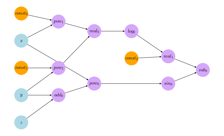
This example, among others, can be seen in the Computational Graphs Notebook in the repository. It’s very recommended that you experiment with these examples and even create your own and visualize them to get a better handle on what’s going on.

Computing Gradients

Now that we have a framework that would allow us to build computational graphs as we go on carrying out our operations, all we need now is something to carry out the actual AD operation: that is something applying the chain rule in breadth-first manner starting form the result node back to the variables nodes. Implementing a breadth-first traversal is as simple as starting from the target node and adding its previous nodes in first-in-first-out queue and then applying the same operation on the front node in the queue until the it gets empty, i.e. it reaches variable or constant nodes which have no previous nodes.

But before we go on defining a method applying that breadth-first traversal, we need a way to define the gradients of the diverse set of operations we have in a consistent way that would allow the traversal method to easily get the desired gradients (or adjoint) once it identified the operation’s name. We can do this by standardizing the way we define our gradients method for all the operations we have, hence providing a consistent interface for the traversal method to use without change across all possible operation nodes.

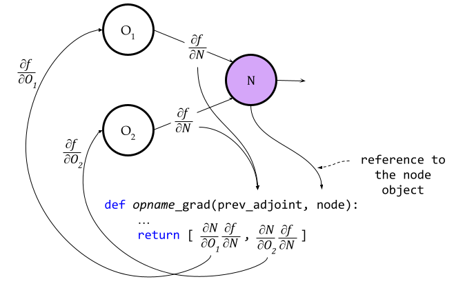
The figure above depicts a way to standardize the gradients method: for each operation we define a method with the name opname_grad where opname is the operations name as its defined in the compgraph package (like add, div, sum, dot, … etc). This method should take two arguments and returns a list of two objects: it should take the node’s adjoint and the node object itself, and it should return the adjoints of its operand nodes; if it’s a unary operation taking only one operand, then the other adjoint should be None. For example, the multiplication operation could be simply defined as:

def mul_grad(prev_adjoint, node):
    return [
        prev_adjoint * node.operand_b,
        prev_adjoint * node.operand_a
    ]

Most of the gradient methods are just a simple application of the chain rule along with the basic differentiation operations like we see in mul_grad. However, when it comes to dealing with multi-dimensional arrays operations provided by numpy’s ndarray, things can get a little tricky! For our purposes here, we can distinguish between two types operations that deal with the ndarrays: reduction and arithmetic operations.

Reduction Operations

In reduction operations, we take an ndarray and reduce it another form, possibly a smaller form, of it. An obvious example of that operations is the sum operation, which takes the whole array and reduce it to a single value representing the summation of its elements. Another one is the max operation that reduces the array to only the maximum value among the elements. The key point in defining the gradients of such operations is realizing that only the elements that contribute to the value of the operation should have a non-zero derivative; the value of these derivatives is then defined by the arithmetic of the reduction operation itself.

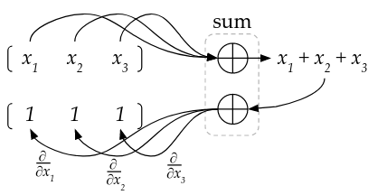
For example, as we see in the figure above, the arithmetic of the sum operation is pretty trivial; we just sum all the elements and output the result of that sum. This makes it easy to show that the derivative of the output w.r.t each element of the array is 1. Now we can simply write the gradient method for sum like the following:

def sum_grad(prev_adjoint, node):
    return [prev_adjoint * np.ones_like(node.operand_a), None]

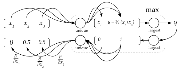
Another example for a reduction operation is the max operation. We can think of the max operation as a function that implements the following pipeline:

1. Extract the unique values from the array by grouping all the same numbers, summing them and then dividing the sum over their count.
2. Output the largest value from the unique values.

So for example, if we want to find the maximum of [1, 4, 4], we extract the unique values as [1/1, (4 + 4) / 2], which is [1, 4] and then output 4 as our max. Following that logic and as the figure above shows, we can get the derivative of the max w.r.t. to each element of the array by following the arithmetic operations that generated our output. In our case here, our output $y$ is the value of $x_2$, which is also the value of $x_3$, so:

From that arithmetic pipeline, we can see that the derivative of the max function w.r.t to some element in the input array is $\frac{1}{\text{max value occurrences count}}$ if that element is the same as the max value, and $0$ otherwise.

From these arithmetic representations of the max operations, we can write its compgraph operation and its gradient methods like the following:

def max(array, axis=None, keepdims=False, name=None):
    if not isinstance(array, Node):
        array = ConstantNode.create_using(array)
    opvalue = np.max(array, axis=axis, keepdims=keepdims)
    opnode = OperationalNode.create_using(opvalue, 'max', array, name=name)

    return opnode

def max_grad(prev_adjoint, node):
    doperand_a = np.where(node.operand_a == node, 1, 0)
    normalizers = np.sum(doperand_a, keepdims=True)
    normalized_doperand_a = doperand_a / normalizers

    return [prev_adjoint * normalized_doperand_a, None]

We can see by running the following snippet that the our gradient calculation is working correctly for something like the array [1, 4, 4] we had earlier (this example and the ones following it can be found in the Gradient Trials notebook):

x = cg.variable(np.array([1, 4, 4]))
max_x = max(x)
print(max_grad(1., max_x))  # prints [array([0. , 0.5, 0.5]), None]

But when we try it for something like [[0, 1, 4], [0, 7, 1]] we find that it doesn’t give a correct answer:

x = cg.variable(np.array([[0, 1, 4], [0, 7, 1]]))
max_x = max(x, axis=0)
print(max_x) # prints [0, 7, 4]

"""
prints
[array([[0.25, 0.  , 0.25],
        [0.25, 0.25, 0.  ]]), None]
while it should print
[array([[0.5, 0, 1],
        [0.5, 1, 0]]), None]
"""
print(max_grad(1, max_x))

To see that the result above is incorrect, we can visualize the gradient of our array along the first axis using the decomposition diagram we used earlier:

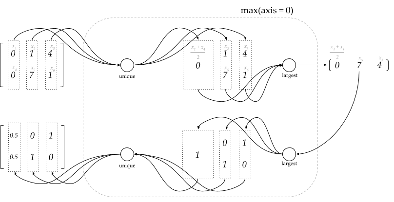
As we can see from the diagram above, the unique operator is applied along the specified axis (which is the first in this case), this change should reflect on how we calculate the normalizers in the gradient method; instead of summing over the whole doperand_a array, we should sum along the specified axis only. This requires the gradient method to know the axis along which the original max operation was performed. We can achieve that by saving this info as an attribute in the node itself while we create it. So we modify our max function and its gradient accordingly:

def max(array, axis=None, keepdims=False, name=None):
    if not isinstance(array, Node):
        array = ConstantNode.create_using(array)
    opvalue = np.max(array, axis=axis, keepdims=keepdims)
    opnode = OperationalNode.create_using(opvalue, 'max', array, name=name)

    # save info for gradient computation
    opnode.axis = axis

    return opnode

def max_grad(prev_adjoint, node):
    doperand_a = np.where(node.operand_a == node, 1, 0)
    normalizers = np.sum(doperand_a, axis=node.axis, keepdims=True)
    normalized_doperand_a = doperand_a / normalizers

    return [prev_adjoint * normalized_doperand_a, None]

With this modification, we can see that the previously incorrect gradient is now calculated correctly. Now, let’s change our max axis to 1 to make sure that everything works smoothly and as expected:

max_x_1 = max(x, axis=1)
print(max_x_1)  # prints [4, 7]

# throws a warning that elementwise comparison failed then raises an error
print(max_grad(1., max_x_1))

Unfortunately, everything is not working smoothly yet. when we shift the axis to 1, we get a warning and an error. The warning says that the elementwise comparison failed, and then an an AxisError is raised at the second line of max_grad where we sum the doperand_a, so the warning must have occurred at the first line of the function, the one with the np.where statement. If we looked closely, our operand x has a shape (2,3), while the max value (the node itself) has a shape (2,). Comparing these two would fail due to incompatible shapes, so the np.where would just return a 0, a scalar with no dimensions at all, which in turn would raise an error at the np.sum statement because we’re trying to sum along the second axis of a scalar that has no axes at all. This can be solved by comparing the operand with a version of the node’s value where the dimensions are kept intact using keepdims=True argument; this would make the node’s value to be of shape (2,1) which can be broadcasted along the operand’s shape. We implement this the same way we did with the axis information, by saving a value of the max operation with the dimensions kept intact as an attribute in the node.

def max(array, axis=None, keepdims=False, name=None):
    if not isinstance(array, Node):
        array = ConstantNode.create_using(array)
    opvalue = np.max(array, axis=axis, keepdims=keepdims)
    opnode = OperationalNode.create_using(opvalue, 'max', array, name=name)

    # save info for gradient computation
    opnode.axis = axis
    opnode.with_keepdims = np.max(array, axis=axis, keepdims=True)

    return opnode

def max_grad(prev_adjoint, node):
    doperand_a = np.where(node.operand_a == node.with_keepdims, 1, 0)
    normalizers = np.sum(doperand_a, axis=node.axis, keepdims=True)
    normalized_doperand_a = doperand_a / normalizers

    return [prev_adjoint * normalized_doperand_a, None]

After that change, we can verify that our gradient works correctly on the second axis and every other possible combinations of parameters.

Implementing gradients for other reduction operations goes the same way we went with the sum and max operations: you just need to understand how these operations are working internally, and pay attention to the shapes. It’s recommended that you take a look at the gards.py file where all the gradient methods are implemented and check how other reduction operations gradients are implemented.

Arithmetic Operations

For most of the arithmetic operations involving multi-dimensional arrays, it’s fairly easy to provide a gradient method. We have seen an example of that earlier with mul_grad for elementwise multiplication. We can see another example for the gradient of elementwise division defined as:

def div_grad(prev_adjoint, node):
    return [
        prev_adjoint / node.operand_b,
        -1 * prev_adjoint * node.operand_a / node.operand_b ** 2
    ]

However, it can get a little tricky when we deal with more specialized operations that work on matrices or multi-dimensional arrays in general. We’ll take matrix multiplication as an example here as it’s considered the most critical operation in neural networks and deep learning. Let’s assume that we have 3 matrices $Y, X$ and $W$. where $X$ is of shape $n \times m$, $W$ is of shape $m \times d$, $Y$ is of shape $n \times d$, and:

We can easily draw parallels between these 3 matrices and neural networks by thinking about the matrix $X$ as the minibatch of size $n$ coming from the previous layer of the network, and $Y$ represents the pre-activations of the current layer with the weights $W$. Let’s also assume that we have real-valued $f = f(Y)$ that depends on $Y$. We can think of this function as the loss function for our model. Given that we know the adjoint $\frac{\partial f}{\partial Y}$, we need to calculate the derivative of $f$ w.r.t $X$ and $W$. Well, this shouldn’t be tricky, we can just apply the chain rule and obtain:

It’s starts getting tricky from here! The problems start to arise when we attempt to calculate the derivatives of $Y$ w.r.t $X$ and $W$. Let’s attempt to calculate $\frac{\partial Y}{\partial W}$ in the special case where both $Y$ and $W$ are both of the shape $2\times 2$. To take the derivative of a matrix with respect to some variable is the same as taking the derivative of each element of the matrix with respect to that same variable. Which translates $\frac{\partial Y}{\partial W}$ into:

Which is not bad so far. However, we need to remember that $W$ is a matrix as well, and to take the derivative of a scalar like $y_{11}$ with respect to a matrix is equivalent to taking the derivative of that scalar with respect to each and every single element of that matrix. So for example, the derivative of $y_{11}$ with respect to $W$ would be:

By doing the same for the other elements of $Y$ and substituting that back to the expression of $\frac{\partial Y}{\partial W}$, we end up with this baby monster:

This baby monster is a matrix of matrices, a.k.a a 4th-rank tensor (or a 4D array). This tensor has $2\times 2\times 2\times 2 = 16$ elements, which seems manageable, but don’t let its small size fool you. Once this monster grows up, it can easily eat up all your computation hardware! For the general case where $Y$ and $W$ are of shapes $n\times d$ and $m\times d$, this derivative tensor will contain $n\times m\times d^{2}$ elements. So for a setting where $n = 32$, $m = 784$, and $d=1024$ (which is a common setting for a neural network layer), we end up with $26306674688$ elements in the derivative tensor. If each of these elements is stored as 32-bit floating number in memory, we’d need around $3GB$ of memory to store that tensor alone. If this is a neural network layer and you have 100 of them, you’d need $300GB$ to get the gradient with respect to a single variable. This is obviously unmanageable. An experienced reader would probably notice that a lot of values in that derivative tensor are zeros, which allows us to treat it as a sparse data structure and store it with a significantly lower memory footprint. While this is technically true, we’ll quickly run into troubles when we try to apply mathematical operations on that sparse 4D array. Sparse structures are notoriously difficult to operate on efficiently, and most of the advances made (either in theory or in hardware support) are made especially for sparse matrices (2D arrays), not general multi-dimensional array. That’s why we see only sparse matrices in scipy and no sparse ndarrays..

Luckily for us, there is a much cheaper way that we can use to calculate the derivatives of $f$ with respect to $W$ and $X$ without the need to compute these monstrous tensors at all. We can simply use:

Seems magical, isn’t it? Well, it’s not, it’s just math. A proof of these equations can be found in the project’s Github repository. It’s a really simple proof but it will make dealing with matrix derivatives less scary, so I suggest that you give it a read. If you’re not interested in the details behind these equations and you trust me on this, I invite you to convince yourself that these equations are true by checking the shapes of all the matrices involved and verify that everything matches. Once you’re convinced, we easily implement the dot_grad method as follows:

def dot_grad(prev_adjoint, node):
    prev_adj = prev_adjoint
    op_a = node.operand_a
    op_b = node.operand_b

    return [
        cg.dot(prev_adj, op_b.T),
        cg.dot(op_a.T, prev_adj)
    ]

We’re now mostly ready to implement the BFS algorithm that will calculate the gradients in any given computational graph. We just need to deal with one caveat introduced by one of numpy’s most powerful features; broadcasting.

Unbroadcasting Adjoints

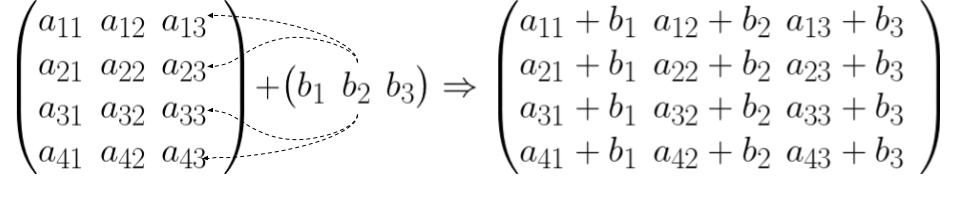
Let’s now consider the equation $Y = XW + b$. This equation is what the pre-activations of a neural network layer looks like after adding the bias vector $b$. In such operation, $XW$ would be a matrix of shape $n\times d$ and the bias is just a vector of shape $d$. When we add the two, numpy broadcasts the vector $b$ across the $n$ rows of $XW$. In other words, it makes $n$ copies of $b$ and add each of these copies to one row of $XW$. Let’s denote the product $XW$ with a single matrix called $A$, so the euqation would turn into $Y=A+b$, the figure below depicts how this process works on when $A$ has shape a $4\times 3 $ and $b$ has a size $3$.

This page of numpy documentation contains more examples on how broadcasting works, but the main idea is the same:

Smaller arrays are [distributed] across the larger array so that they have compatible shapes.

Broadcasting is a very handy feature that makes carrying out array operations efficient. However, that same handy feature poses a problem when we try to do automatic differentiation. To compute $\frac{\partial f}{\partial b}$, we simply apply the chain rule and get:

Which means that the derivative of $f$ with respect to $b$ is the same as the derivative of $f$ with respect to $Y$. We know that we need $\frac{\partial f}{\partial b}$ to be of the same shape as $b$ itself in order to do something like gradient decent updates. In other words, we need $\frac{\partial f}{\partial b}$ to be a vector of size $d$ as well. However, we’re getting a matrix of shape $n\times d$ instead. This difference in expected shape happened because numpy has broadcasted $b$ across $XW$ to get $Y$, and if we want to get the shapes right, we need to undo that broadcasting when we calculate the adjoint at $b$.

The idea behind unbroadcasting becomes very simple once we try to visualize what happened in terms of a computational graph. Let’s get back to the figure above and assume that $R_1,R_2,R_3$ and $R_4$ are the four rows of the matrix $A$. We saw that broadcasting $b$ across $A$ happens by adding $b$ to each row of $A$, so one could argue that the following two computational graphs are the same.

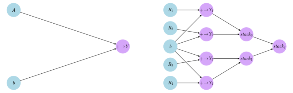
In the graphs above, $+ \rightarrow Y_i$ means that the addition of two operands yield the $i^{th}$ row of $Y$. Moreover, we assume that we have a stack operation that simply stacks the two inputs on top of each other in the correct order. It’s not hard to see that both graphs yield the same matrix. However, the graph on the right has the advantage of calculating the adjoint at $b$ in the right shape. We see that $b$ is contributing to multiple nodes in the graph, so the multivariable chain rule will apply and we get:

All the derivatives with respect to $b$ in the terms on the right hand side would evaluate to $1$, which leaves us with:

Which is correctly a vector of size $d$. Now remember that both computational graphs above are identical, which means we can transfer what we learned from the right graph to the left one, and this gives us the key to how we can unbroadcast adjoints into their original shape. So to get the adjoint $\frac{\partial f}{\partial b}$ correctly out of the adjoint $\frac{\partial f}{\partial Y}$, we need to sum out all the $n$ rows from $\frac{\partial f}{\partial Y}$.

This simple idea of unbroadcasting (which is just the multivariable chain rule in disguise) applies to all broadcasting patterns supported by numpy and can be summarized in very tiny algorithm

All the extra dimensions that the adjojnt have over the original node shape should be summed out. For each of the remaining dimensions, if the size of the original dimension in the node is 1, this dimension should be summed out too but its place should be preserved

This tiny algorithm translates to the following small python code:

def unbroadcast_adjoint(node, adjoint):

    correct_adjoint = adjoint

    if node.shape != adjoint.shape:
        dimensions_diff = np.abs(adjoint.ndim - node.ndim)
        if dimensions_diff != 0:
            summation_dims = tuple(range(dimensions_diff))
            correct_adjoint = cg.sum(adjoint, axis=summation_dims)

            originally_ones = tuple([axis if size == 1 for axis, size in enumerate(node.shape)])
            if len(originally_ones) != 0:
                correct_adjoint = cg.sum(correct_adjoint, axis=axis, keepdims=True)

    return correct_adjoint

Putting Everything Into Action

With the unbroadcast_adjoint method in our hands, we have all the pieces needed to build our BFS algorithm calculating the gradient of a computational graph. The implementation is actually very simple: we use an iterative implementation of BFS using a queue that initially contains the last node of the computational graph. Then we run the following until the queue is empty:

1. Pop the first node in the queue
2. If the node is a constant, do nothing and continue the loop
3. If the node is a variable, set the derivative with respect to this variable to the adjoint associated with the node
4. If the node is an operational node, do:
   • 4.1. Obtain the gradient method for this operation and calculate the gradient of the node w.r.t its operands and update the operands adjoints
   • 4.2 Apply unbroadcasting to the updated operands adjoints
   • 4.3 Enqueue the operands of the current node

The implementation can be found in the autodiff/reverse.py module, it’s just a python translation of the procedure outlined above with some helper data structures. This module also has a check_gradient method which uses the definition of a derivative as limit to approximate the gradients of a function (we worked with a similar method in the first part with forward mode AD). We could use this checker method to verify that our implementation of reverse mode AD is actually correct. We’ll try with a small function of three variables $f(x,y,z) = \sin(x^{y + z}) - 3\ln(x^2y^3)$ at $(x, y, z) = (0.5, 4, -2.3)$.

def func(x,y,z):
    _x = cg.variable(x, 'x')
    _y = cg.variable(y, 'y')
    _z = cg.variable(z, 'z')

    return  cg.sin(_x ** (_y + _z)) - 3 * _z * cg.log((_x ** 2) * (_y ** 3))

f = func(0.5, 4, -2.3)
g = gradient(f)

# prints "Gradient Checking Result: True"
print("Gradient Checking Result: {}".format(
    check_gradient(
        func,
        [0.5, 4, -2.3],
        [g[v] for v in ('x', 'y', 'z')]
    )
))

Training a Neural Network

This is the moment we’re all have been waiting for, to use everything we built so far and build ourselves a fully functional neural network. We’ll build our network to classify images of handwritten digits using the famous MNIST dataset. We’ll start by fetching the dataset using scikit-learn, preprocess it and split it into a training and test sets.

from sklearn.utils import shuffle
from sklearn.datasets import fetch_openml
from sklearn.preprocessing import LabelBinarizer
from sklearn.model_selection import train_test_split
import numpy as np

X, y = fetch_openml('mnist_784', version=1, return_X_y=True, as_frame=False)
label_binarizer = LabelBinarizer()

# transforming all geryscale values to range [0,1]
# 0 being black and 1 beiung white 
X_scaled = X / 255

# transfrom categorical target labels into one-vs-all fashion
y_binarized = label_bin.fit_transform(y)

# splitting the data to 80% training and 20% testing
X_train, X_test, y_train, y_test = train_test_split(X_scaled, y_binarized, test_size=0.2, random_state=42)

We’ll now use the compgraph module to build a two layers neural networks with a ReLU activation.

import compgraph as cg

def relu(x):
    return cg.where(x > 0, x, 0)

l1_weights = cg.variable(np.random.normal(scale=np.sqrt(2./784), size=(784, 64)), name='l1_w')
l1_bias = cg.variable(np.zeros(64), name='l1_b')
l2_weights = cg.variable(np.random.normal(scale=np.sqrt(2./64), size=(64, 10)), name='l2_w')
l2_bias = cg.variable(np.zeros(10), name='l2_b')


def nn(x):
    l1_activations = relu(cg.dot(x, l1_weights) + l1_bias)
    l2_activations = cg.dot(l1_activations, l2_weights) + l2_bias
    
    return l2_activations

To train this small neural net we just built, we’ll simply implement a training loop that samples a batch of 32 images and passes them to the nn function. With the outputs of the nn function and the target labels we have, we’ll compute the softmax_cross_entropy loss and use the gradient method from autodiff.reverse to compute the gradient of that loss with respect to the network’s variables. Once we have the gradients, we easily update the weights and the biases using the gradient descent update rule:

from tqdm import trange

from autodiff.reverse import gradient

LEARNING_RATE = 0.01
BATCH_SIZE = 32
ITERATIONS = 50000

last1000_losses = []
progress_bar = trange(ITERATIONS)
training_set_pointer = 0

for i in progress_bar:
    batch_x = X_train[training_set_pointer:training_set_pointer + BATCH_SIZE]
    batch_y = y_train[training_set_pointer:training_set_pointer + BATCH_SIZE]
    
    if training_set_pointer + BATCH_SIZE >= len(y_train):
        # if the training set is consumed, start from the beginning
        training_set_pointer = 0
    else:
        training_set_pointer += BATCH_SIZE
    
    logits = nn(batch_x)
    loss = cg.softmax_cross_entropy(logits, batch_y)
    last1000_losses.append(loss)
    
    progress_bar.set_description(
        "Avg. Loss (Last 1k Iterations): {:.5f}".format(np.mean(last1000_losses))
    )
    
    if len(last1000_losses) == 1000:
        last1000_losses.pop(0)
    
    grads = gradient(loss)
    
    l1_weights -= learning_rate * grads['l1_w']
    l2_weights -= learning_rate * grads['l2_w']
    l1_bias -= learning_rate * grads['l1_b']
    l2_bias -= learning_rate * grads['l2_b']

We use the tqdm library in this training loop to show a progress bar of the training iterations along with the average loss in the last 1000 iterations. When we run this training loop, we’ll actually find that the loss is decreasing and the network will converge to a very small error (around $6 \times 10^{-5}$), which means that the network is learning effectively. To verify that, we can test the network on the held-out test set and check its accuracy.

def softmax(x, axis):
    x_max = cg.max(x, axis=axis, keepdims=True)
    exp_op = cg.exp(x - x_max)
    return exp_op/ cg.sum(exp_op, axis=axis, keepdims=True)

logits = nn(X_test)
probabilities = softmax(logits, axis=-1)
predicted_labels = np.argmax(probabilities, axis=-1)
true_labels = np.argmax(y_test, axis=-1)
accuracy = np.mean(predicted_labels == true_labels)

# prints something around 97%
print("Accuracy: {:.2f}%".format(accuracy * 100))

By running this test script (which can be found in the [Reverse AD notebook] in the repository, along with all the other previous scripts), we can see that the network did learn well with an accuracy 97%!

Avoiding Numerical Instability

You may have noticed in the training loop script above, we used a cg.softmax_cross_entropy to calculate the loss instead of implementing the softmax and cross-entropy functions from the other primitives. The reason behind that can be revelead by looking at how our framework would compute the gradients of the loss with respect to the logits when we implement softmax and cross-entropy loss sperately. Let’s assume that the $i^{th}$ logit outtpted from the neural network is denoted by $l_i$. To calculate the loss, we first apply softmax on the logits vector and then use the cross-entropy between the targets and softmax outputs. That is:

Hence, to calculate the derivative of the loss with respect to the logits, our framework apply the rule and have:

The framework would calculate ecah of the derivatives on the right hand side seperatly and then simply multiply them. So first, the framework would calculate the derivative of the loss w.r.t $s_i$ to be:

And no matter what the other derivative is, the chain rule application will be:

Rememberthat the value of $s_i$ lies between 0 and 1 and it can be easily very small when we have more classes in the data. With this in mind, we can quickly understand why this multiplication is problematic. Because $s_i$ can be arbitrarly small, this multiplication is prone to overflow and generate infinities or NaNs (not a number). An operation of such charataristic is said to be numerically instable.

On the other hand, if we calculted the derivative of the softmax and combined the both by hand, we get a very stable and neat expression for the $\frac{\partial L}{\partial l_i}$:

Because this operation is numerically stable, softmax_cross_entropy is treated as a primitive operation of its own with its gradient being the stable $s - y$ operation. To cement this result, I invite you to implement the two operation spearatly and try to train the neural network with it and see how the loss quickly turns nan.

Congrats!

Congratulations! You have finished your own deep learning framwork and succefully trained a neural network with it! It’s been a long journey, but we made it through. I hope that now you know how the magic behind these famous frameworks really works, and now you can fully harnness these magical powers to your service.

Thanks a lot fot reading!

References

• Backpropagation for a Linear Layer, by Justin Johnson. A Stanford’s CS231n Handout
• HIPS/autoghrad Sourcecode