Machine Learning Theory - Part 2: Generalization Bounds

Last time we concluded by noticing that minimizing the empirical risk (or the training error) is not in itself a solution to the learning problem, it could only be considered a solution if we can guarantee that the difference between the training error and the generalization error (which is also called the generalization gap) is small enough. We formalized such requirement using the probability:

That is if this probability is small, we can guarantee that the difference between the errors is not much, and hence the learning problem can be solved.

In this part we’ll start investigating that probability at depth and see if it indeed can be small, but before starting you should note that I skipped a lot of the mathematical proofs here. You’ll often see phrases like “It can be proved that …”, “One can prove …”, “It can be shown that …”, … etc without giving the actual proof. This is to make the post easier to read and to focus all the effort on the conceptual understanding of the subject. In case you wish to get your hands dirty with proofs, you can find all of them in the additional readings, or on the Internet of course!

Independently, and Identically Distributed

The world can be a very messy place! This is a problem that faces any theoretical analysis of a real world phenomenon; because usually we can’t really capture all the messiness in mathematical terms, and even if we’re able to; we usually don’t have the tools to get any results from such a messy mathematical model.

So in order for theoretical analysis to move forward, some assumptions must be made to simplify the situation at hand, we can then use the theoretical results from that simplification to infer about reality.

Assumptions are common practice in theoretical work. Assumptions are not bad in themselves, only bad assumptions are bad! As long as our assumptions are reasonable and not crazy, they’ll hold significant truth about reality.

A reasonable assumption we can make about the problem we have at hand is that our training dataset samples are independently, and identically distributed (or i.i.d. for short), that means that all the samples are drawn from the same probability distribution and that each sample is independent from the others.

This assumption is essential for us. We need it to start using the tools form probability theory to investigate our generalization probability, and it’s a very reasonable assumption because:

1. It’s more likely for a dataset used for inferring about an underlying probability distribution to be all sampled for that same distribution. If this is not the case, then the statistics we get from the dataset will be noisy and won’t correctly reflect the target underlying distribution.
2. It’s more likely that each sample in the dataset is chosen without considering any other sample that has been chosen before or will be chosen after. If that’s not the case and the samples are dependent, then the dataset will suffer from a bias towards a specific direction in the distribution, and hence will fail to reflect the underlying distribution correctly.

So we can build upon that assumption with no fear.

The Law of Large Numbers

Most of us, since we were kids, know that if we tossed a fair coin a large number of times, roughly half of the times we’re gonna get heads. This is an instance of wildly known fact about probability that if we retried an experiment for a sufficiency large amount of times, the average outcome of these experiments (or, more formally, the sample mean) will be very close to the true mean of the underlying distribution. This fact is formally captured into what we call The law of large numbers:

If $x_1, x_2, …, x_m$ are $m$ i.i.d. samples of a random variable $X$ distributed by $P$. then for a small positive non-zero value $\epsilon$:

\[\lim_{m \rightarrow \infty} \mathbb{P}\left[\left|\mathop{\mathbb{E}}_{X \sim P}[X] - \frac{1}{m}\sum_{i=1}^{m}x_i \right| > \epsilon\right] = 0\]

This version of the law is called the weak law of large numbers. It’s weak because it guarantees that as the sample size goes larger, the sample and true means will likely be very close to each other by a non-zero distance no greater than epsilon. On the other hand, the strong version says that with very large sample size, the sample mean is almost surely equal to the true mean.

The formulation of the weak law lends itself naturally to use with our generalization probability. By recalling that the empirical risk is actually the sample mean of the errors and the risk is the true mean, for a single hypothesis $h$ we can say that:

Well, that’s a progress, A pretty small one, but still a progress! Can we do any better?

Hoeffding’s inequality

The law of large numbers is like someone pointing the directions to you when you’re lost, they tell you that by following that road you’ll eventually reach your destination, but they provide no information about how fast you’re gonna reach your destination, what is the most convenient vehicle, should you walk or take a cab, and so on.

To our destination of ensuring that the training and generalization errors do not differ much, we need to know more info about the how the road down the law of large numbers look like. These info are provided by what we call the concentration inequalities. This is a set of inequalities that quantifies how much random variables (or function of them) deviate from their expected values (or, also, functions of them). One inequality of those is Heoffding’s inequality:

If $x_1, x_2, …, x_m$ are $m$ i.i.d. samples of a random variable $X$ distributed by $P$, and $a \leq x_i \leq b$ for every $i$, then for a small positive non-zero value $\epsilon$:

\[\mathbb{P}\left[\left|\mathop{\mathbb{E}}_{X \sim P}[X] - \frac{1}{m}\sum_{i=0}^{m}x_i\right| > \epsilon\right] \leq 2\exp\left(\frac{-2m\epsilon^2}{(b -a)^2}\right)\]

You probably see why we specifically chose Heoffding’s inequality from among the others. We can naturally apply this inequality to our generalization probability, assuming that our errors are bounded between 0 and 1 (which is a reasonable assumption, as we can get that using a 0/1 loss function or by squashing any other loss between 0 and 1) and get for a single hypothesis $h$:

This means that the probability of the difference between the training and the generalization errors exceeding $\epsilon$ exponentially decays as the dataset size goes larger. This should align well with our practical experience that the bigger the dataset gets, the better the results become.

If you noticed, all our analysis up till now was focusing on a single hypothesis $h$. But the learning problem doesn’t know that single hypothesis beforehand, it needs to pick one out of an entire hypothesis space $\mathcal{H}$, so we need a generalization bound that reflects the challenge of choosing the right hypothesis.

Generalization Bound: 1st Attempt

In order for the entire hypothesis space to have a generalization gap bigger than $\epsilon$, at least one of its hypothesis: $h_1$ or $h_2$ or $h_3$ or … etc should have. This can be expressed formally by stating that:

Where $\bigcup$ denotes the union of the events, which also corresponds to the logical OR operator. Using the union bound inequality, we get:

We exactly know the bound on the probability under the summation from our analysis using the Heoffding’s inequality, so we end up with:

Where $|\mathcal{H}|$ is the size of the hypothesis space. By denoting the right hand side of the above inequality by $\delta$, we can say that with a confidence $1 - \delta$:

And with some basic algebra, we can express $\epsilon$ in terms of $\delta$ and get:

This is our first generalization bound, it states that the generalization error is bounded by the training error plus a function of the hypothesis space size and the dataset size. We can also see that the the bigger the hypothesis space gets, the bigger the generalization error becomes. This explains why the memorization hypothesis form last time, which theoretically has $|\mathcal{H}| = \infty$, fails miserably as a solution to the learning problem despite having $R_\text{emp} = 0$; because for the memorization hypothesis $h_\text{mem}$:

But wait a second! For a linear hypothesis of the form $h(x) = wx + b$, we also have $|\mathcal{H}| = \infty$ as there is infinitely many lines that can be drawn. So the generalization error of the linear hypothesis space should be unbounded just as the memorization hypothesis! If that’s true, why does perceptrons, logistic regression, support vector machines and essentially any ML model that uses a linear hypothesis work?

Our theoretical result was able to account for some phenomena (the memorization hypothesis, and any finite hypothesis space) but not for others (the linear hypothesis, or other infinite hypothesis spaces that empirically work). This means that there’s still something missing from our theoretical model, and it’s time for us to revise our steps. A good starting point is from the source of the problem itself, which is the infinity in $|\mathcal{H}|$.

Notice that the term $|\mathcal{H}|$ resulted from our use of the union bound. The basic idea of the union bound is that it bounds the probability by the worst case possible, which is when all the events under union are mutually independent. This bound gets more tight as the events under consideration get less dependent. In our case, for the bound to be tight and reasonable, we need the following to be true:

For every two hypothesis $h_1, h_2 \in \mathcal{H}$ the two events $|R(h_1) - R_\text{emp}(h_1)| > \epsilon$ and $|R(h_2) - R_\text{emp}(h_2)| > \epsilon$ are likely to be independent. This means that the event that $h_1$ has a generalization gap bigger than $\epsilon$ should be independent of the event that also $h_2$ has a generalization gap bigger than $\epsilon$, no matter how much $h_1$ and $h_2$ are close or related; the events should be coincidental.

But is that true?

Examining the Independence Assumption

The first question we need to ask here is why do we need to consider every possible hypothesis in $\mathcal{H}$? This may seem like a trivial question; as the answer is simply that because the learning algorithm can search the entire hypothesis space looking for its optimal solution. While this answer is correct, we need a more formal answer in light of the generalization inequality we’re studying.

The formulation of the generalization inequality reveals a main reason why we need to consider all the hypothesis in $\mathcal{H}$. It has to do with the existence of $\sup_{h \in \mathcal{H}}$. The supremum in the inequality guarantees that there’s a very little chance that the biggest generalization gap possible is greater than $\epsilon$; this is a strong claim and if we omit a single hypothesis out of $\mathcal{H}$, we might miss that “biggest generalization gap possible” and lose that strength, and that’s something we cannot afford to lose. We need to be able to make that claim to ensure that the learning algorithm would never land on a hypothesis with a bigger generalization gap than $\epsilon$.

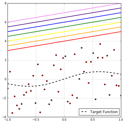
Looking at the above plot of binary classification problem, it’s clear that this rainbow of hypothesis produces the same classification on the data points, so all of them have the same empirical risk. So one might think, as they all have the same $R_\text{emp}$, why not choose one and omit the others?!

This would be a very good solution if we’re only interested in the empirical risk, but our inequality takes into its consideration the out-of-sample risk as well, which is expressed as:

This is an integration over every possible combination of the whole input and output spaces $\mathcal{X, Y}$. So in order to ensure our supremum claim, we need the hypothesis to cover the whole of $\mathcal{X \times Y}$, hence we need all the possible hypotheses in $\mathcal{H}$.

Now that we’ve established that we do need to consider every single hypothesis in $\mathcal{H}$, we can ask ourselves: are the events of each hypothesis having a big generalization gap are likely to be independent?

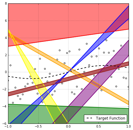
Well, Not even close! Take for example the rainbow of hypotheses in the above plot, it’s very clear that if the red hypothesis has a generalization gap greater than $\epsilon$, then, with 100% certainty, every hypothesis with the same slope in the region above it will also have that. The same argument can be made for many different regions in the $\mathcal{X \times Y}$ space with different degrees of certainty as in the following figure.

But this is not helpful for our mathematical analysis, as the regions seems to be dependent on the distribution of the sample points and there is no way we can precisely capture these dependencies mathematically, and we cannot make assumptions about them without risking to compromise the supremum claim.

So the union bound and the independence assumption seem like the best approximation we can make,but it highly overestimates the probability and makes the bound very loose, and very pessimistic!

However, what if somehow we can get a very good estimate of the risk $R(h)$ without needing to go over the whole of the $\mathcal{X \times Y}$ space, would there be any hope to get a better bound?

The Symmetrization Lemma

Let’s think for a moment about something we do usually in machine learning practice. In order to measure the accuracy of our model, we hold out a part of the training set to evaluate the model on after training, and we consider the model’s accuracy on this left out portion as an estimate for the generalization error. This works because we assume that this test set is drawn i.i.d. from the same distribution of the training set (this is why we usually shuffle the whole dataset beforehand to break any correlation between the samples).

It turns out that we can do a similar thing mathematically, but instead of taking out a portion of our dataset $S$, we imagine that we have another dataset $S’$ with also size $m$, we call this the ghost dataset. Note that this has no practical implications, we don’t need to have another dataset at training, it’s just a mathematical trick we’re gonna use to git rid of the restrictions of $R(h)$ in the inequality.

We’re not gonna go over the proof here, but using that ghost dataset one can actually prove that:

where $R_\text{emp}’(h)$ is the empirical risk of hypothesis $h$ on the ghost dataset. This means that the probability of the largest generalization gap being bigger than $\epsilon$ is at most twice the probability that the empirical risk difference between $S, S’$ is larger than $\frac{\epsilon}{2}$. Now that the right hand side in expressed only in terms of empirical risks, we can bound it without needing to consider the the whole of $\mathcal{X \times Y}$, and hence we can bound the term with the risk $R(h)$ without considering the whole of input and output spaces!

This, which is called the symmetrization lemma, was one of the two key parts in the work of Vapnik-Chervonenkis (1971).

The Growth Function

Now that we are bounding only the empirical risk, if we have many hypotheses that have the same empirical risk (a.k.a. producing the same labels/values on the data points), we can safely choose one of them as a representative of the whole group, we’ll call that an effective hypothesis, and discard all the others.

By only choosing the distinct effective hypotheses on the dataset $S$, we restrict the hypothesis space $\mathcal{H}$ to a smaller subspace that depends on the dataset $\mathcal{H}_{|S}$.

We can assume the independence of the hypotheses in $\mathcal{H}_{|S}$ like we did before with $\mathcal{H}$ (but it’s more plausible now), and use the union bound to get that:

Notice that the hypothesis space is restricted by $S \cup S’$ because we using the empirical risk on both the original dataset $S$ and the ghost $S’$. The question now is what is the maximum size of a restricted hypothesis space? The answer is very simple; we consider a hypothesis to be a new effective one if it produces new labels/values on the dataset samples, then the maximum number of distinct hypothesis (a.k.a the maximum number of the restricted space) is the maximum number of distinct labels/values the dataset points can take. A cool feature about that maximum size is that its a combinatorial measure, so we don’t need to worry about how the samples are distributed!

For simplicity, we’ll focus now on the case of binary classification, in which $\mathcal{Y}=\{-1, +1\}$. Later we’ll show that the same concepts can be extended to both multiclass classification and regression. In that case, for a dataset with $m$ samples, each of which can take one of two labels: either -1 or +1, the maximum number of distinct labellings is $2^m$.

We’ll define the maximum number of distinct labellings/values on a dataset $S$ of size $m$ by a hypothesis space $\mathcal{H}$ as the growth function of $\mathcal{H}$ given $m$, and we’ll denote that by $\Delta_\mathcal{H}(m)$. It’s called the growth function because it’s value for a single hypothesis space $\mathcal{H}$ (aka the size of the restricted subspace $\mathcal{H_{|S}}$) grows as the size of the dataset grows. Now we can say that:

Notice that we used $2m$ because we have two datasets $S,S’$ each with size $m$.

For the binary classification case, we can say that:

But $2^m$ is exponential in $m$ and would grow too fast for large datasets, which makes the odds in our inequality go too bad too fast! Is that the best bound we can get on that growth function?

The VC-Dimension

The $2^m$ bound is based on the fact that the hypothesis space $\mathcal{H}$ can produce all the possible labellings on the $m$ data points. If a hypothesis space can indeed produce all the possible labels on a set of data points, we say that the hypothesis space shatters that set.

But can any hypothesis space shatter any dataset of any size? Let’s investigate that with the binary classification case and the $\mathcal{H}$ of linear classifiers $\mathrm{sign}(wx + b)$. The following animation shows how many ways a linear classifier in 2D can label 3 points (on the left) and 4 points (on the right).

In the animation, the whole space of possible effective hypotheses is swept. For the the three points, the hypothesis shattered the set of points and produced all the possible $2^3 = 8$ labellings. However for the four points,the hypothesis couldn’t get more than 14 and never reached $2^4 = 16$, so it failed to shatter this set of points. Actually, no linear classifier in 2D can shatter any set of 4 points, not just that set; because there will always be two labellings that cannot be produced by a linear classifier which is depicted in the following figure.

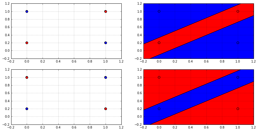
From the decision boundary plot (on the right), it’s clear why no linear classifier can produce such labellings; as no linear classifier can divide the space in this way. So it’s possible for a hypothesis space $\mathcal{H}$ to be unable to shatter all sizes. This fact can be used to get a better bound on the growth function, and this is done using Sauer’s lemma:

If a hypothesis space $\mathcal{H}$ cannot shatter any dataset with size more than $k$, then:

\[\Delta_{\mathcal{H}}(m) \leq \sum_{i=0}^{k}\binom{m}{i}\]

This was the other key part of Vapnik-Chervonenkis work (1971), but it’s named after another mathematician, Norbert Sauer; because it was independently proved by him around the same time (1972). However, Vapnik and Chervonenkis weren’t completely left out from this contribution; as that $k$, which is the maximum number of points that can be shattered by $\mathcal{H}$, is now called the Vapnik-Chervonenkis-dimension or the VC-dimension $d_{\mathrm{vc}}$ of $\mathcal{H}$.

For the case of the linear classifier in 2D, $d_\mathrm{vc} = 3$. In general, it can be proved that hyperplane classifiers (the higher-dimensional generalization of line classifiers) in $\mathbb{R}^n$ space has $d_\mathrm{vc} = n + 1$.

The bound on the growth function provided by sauer’s lemma is indeed much better than the exponential one we already have, it’s actually polynomial! Using algebraic manipulation, we can prove that:

Where $O$ refers to the Big-O notation for functions asymptotic (near the limits) behavior, and $e$ is the mathematical constant.

Thus we can use the VC-dimension as a proxy for growth function and, hence, for the size of the restricted space $\mathcal{H_{|S}}$. In that case, $d_\mathrm{vc}$ would be a measure of the complexity or richness of the hypothesis space.

The VC Generalization Bound

With a little change in the constants, it can be shown that Heoffding’s inequality is applicable on the probability $\mathbb{P}\left[|R_\mathrm{emp}(h) - R_\mathrm{emp}’(h)| > \frac{\epsilon}{2}\right]$. With that, and by combining inequalities (1) and (2), the Vapnik-Chervonenkis theory follows:

This can be re-expressed as a bound on the generalization error, just as we did earlier with the previous bound, to get the VC generalization bound:

or, by using the bound on growth function in terms of $d_\mathrm{vc}$ as:

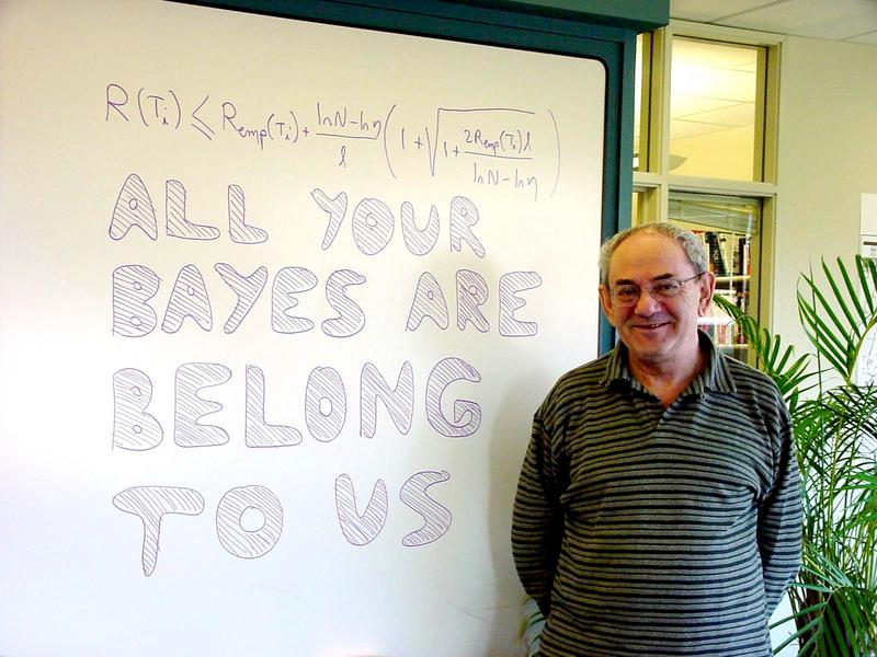
Professor Vapnik standing in front of a white board that has a form of the VC-bound and the phrase “All your bayes are belong to us”, which is a play on the broken english phrase found in the classic video game Zero Wing in a claim that the VC framework of inference is superior to that of Bayesian inference. [Courtesy of Yann LeCunn].

This is a significant result! It’s a clear and concise mathematical statement that the learning problem is solvable, and that for infinite hypotheses spaces there is a finite bound on the their generalization error! Furthermore, this bound can be described in term of a quantity ($d_\mathrm{vc}$), that solely depends on the hypothesis space and not on the distribution of the data points!

Now, in light of these results, is there’s any hope for the memorization hypothesis?

It turns out that there’s still no hope! The memorization hypothesis can shatter any dataset no matter how big it is, that means that its $d_\mathrm{vc}$ is infinite, yielding an infinite bound on $R(h_\mathrm{mem})$ as before. However, the success of linear hypothesis can now be explained by the fact that they have a finite $d_\mathrm{vc} = n + 1$ in $\mathbb{R}^n$. The theory is now consistent with the empirical observations.

Distribution-Based Bounds

The fact that $d_\mathrm{vc}$ is distribution-free comes with a price: by not exploiting the structure and the distribution of the data samples, the bound tends to get loose. Consider for example the case of linear binary classifiers in a very higher n-dimensional feature space, using the distribution-free $d_\mathrm{vc} = n + 1$ means that the bound on the generalization error would be poor unless the size of the dataset $N$ is also very large to balance the effect of the large $d_\mathrm{vc}$. This is the good old curse of dimensionality we all know and endure.

However, a careful investigation into the distribution of the data samples can bring more hope to the situation. For example, For data points that are linearly separable, contained in a ball of radius $R$, with a margin $\rho$ between the closest points in the two classes, one can prove that for a hyperplane classifier:

It follows that the larger the margin, the lower the $d_\mathrm{vc}$ of the hypothesis. This is theoretical motivation behind Support Vector Machines (SVMs) which attempts to classify data using the maximum margin hyperplane. This was also proved by Vapnik and Chervonenkis.

One Inequality to Rule Them All

Up until this point, all our analysis was for the case of binary classification. And it’s indeed true that the form of the vc bound we arrived at here only works for the binary classification case. However, the conceptual framework of VC (that is: shattering, growth function and dimension) generalizes very well to both multi-class classification and regression.

Due to the work of Natarajan (1989), the Natarajan dimension is defined as a generalization of the VC-dimension for multiple classes classification, and a bound similar to the VC-Bound is derived in terms of it. Also, through the work of Pollard (1984), the pseudo-dimension generalizes the VC-dimension for the regression case with a bound on the generalization error also similar to VC’s.

There is also Rademacher’s complexity, which is a relatively new tool (devised in the 2000s) that measures the richness of a hypothesis space by measuring how well it can fit to random noise. The cool thing about Rademacher’s complexity is that it’s flexible enough to be adapted to any learning problem, and it yields very similar generalization bounds to the other methods mentioned.

However, no matter what the exact form of the bound produced by any of these methods is, it always takes the form:

where $C$ is a function of the hypothesis space complexity (or size, or richness), $N$ the size of the dataset, and the confidence $1 - \delta$ about the bound. This inequality basically says the generalization error can be decomposed into two parts: the empirical training error, and the complexity of the learning model.

This form of the inequality holds to any learning problem no matter the exact form of the bound, and this is the one we’re gonna use throughout the rest of the series to guide us through the process of machine learning.

References and Additional Readings

• Mohri, Mehryar, Afshin Rostamizadeh, and Ameet Talwalkar. Foundations of machine learning. MIT press, 2012.
• Shalev-Shwartz, Shai, and Shai Ben-David. Understanding machine learning: From theory to algorithms. Cambridge University Press, 2014.
• Abu-Mostafa, Y. S., Magdon-Ismail, M., & Lin, H. (2012). Learning from data: a short course.