Machine Learning Theory - Part 3: Regularization and the Bias-variance Trade-off

In first part we explored the statistical model underlying the machine learning problem, and used it to formalize the problem in terms of obtaining the minimum generalization error. By noting that we cannot directly evaluate the generalization error of an ML model, we continued in the second part by establishing a theory that relates this elusive generalization error to another error metric that we can actually evaluate, which is the empirical error. Our final result was that:

That is: the generalization error (or the risk) $R(h)$ is bounded by the empirical risk (or the training error) plus a term that is proportionate to the complexity (or the richness) of the hypothesis space $|\mathcal{H}|$, the dataset size $N$, and the degree of certainty $1 - \delta$ about the bound. We can simplify that bound even more by assuming that we have a fixed dataset (which is the typical case in most practical ML problems), so that for a specific degree of certainty we have:

Starting from this part, and based on this simplified theoretical result, we’ll begin to draw some practical concepts for the process of solving the ML problem. We’ll start by trying to get more intuition about why a more complex hypothesis space is bad.

Why rich hypotheses are bad?

To make things a little bit concrete and to be able to visualize what we’re talking about, we’ll be using the help of a simulated dataset which is a useful tool that is used often to demonstrate concepts in which we might need to draw multiple instance of the dataset from the same distribution; something that cannot be effectively done with real datasets. In a simulated dataset we define our own target function, and use that function, through the help of a computer program, to draw as much datasets as we want form the distribution it describes.

In the following discussion we’re gonna to sample $x$ uniformly from the interval $[-1,1]$ and use a one-dimensional target function $f(x) = \sin(x)$ which generates a noisy response (as we discussed in the first part) $y = f(x) + \zeta$ where $\zeta$ is a random noise drawn from a zero-mean distribution, in our case a Gaussian distribution with a standard deviation of 2.

Recall that when we train an ML model on a dataset, we are trying to find the relation between the predictor features $x$ and the response $y$, so ideally we need hypothesis to account for the noise as little as possible; as noise by definition has no explanatory value whatsoever, and accommodation of noise will skew the model away from the true target resulting in poor performance on future data, hence poor generalization. In order to understand the problem of rich hypotheses, we’ll investigate how different hypotheses of different complexities adhere to such criteria.

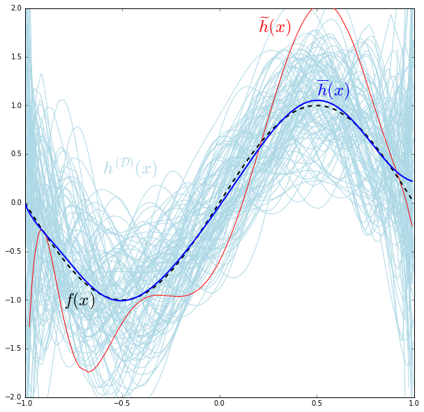
In the following animation we train a linear, a cubic and a tenth degree polynomial hypotheses each on 100 different simulated datasets of 200 points (only 20 are shown) drawn form the above described distribution. Each of these models is drawn with light-blue line, the average of each hypothesis is shown with the darker blue line, while the true target is shown by the dashed black line. The offset of the points from the true target curve is an indicator of the noise; because if there wasn’t any noise, the points would lie on the dashed black curve. So the further the point is from the true target curve, the more noisy it is.

The first thing we notice from that animation is that the richer and more complex the hypothesis gets, the less the its difference from the true target becomes on average. That difference between the estimator’s mean (the hypothesis) and the value it’s trying to estimate (the target) is referred to in statistics as the bias.

Where $\overline{h}(x)$ is the mean of different hypotheses generated from training the model on different datasets, i.e. $\overline{h}(x) = \mathop{\mathbb{E}}_{\mathcal{D}}\left[h^{(\mathcal{D})}(x)\right]$, where $h^{(\mathcal{D})}(x)$ indicates a hypothesis generated by training on the dataset $\mathcal{D}$.

In English, the word “bias” commonly implies some kind of an inclination or prejudice towards something. Analogously, the bias in a statistical estimator can be interpreted as the estimator favoring some specific direction or a component in the target distribution over other major components. To make this interpretation concrete let’s take a look at the Taylor’s expansion of our target function. If you’re not familiar with the concept of Taylor’s expansion, you can think of it method to write a function as a infinite sum of simpler functions, you can consider such simpler functions as components for the sake of our discussion here.

It’s obvious from the increasing value of the denominator that each higher component contributes very little to the value of the function which makes higher components minor and unimportant.

The high bias of the linear model can now be interpreted by the linear hypothesis function $h(x) = w_1x + w_0$ favoring the $x$ component of the target over the other major component $\frac{x^3}{3!}$. With the same logic, the seemingly low bias of cubic model can be explained by the fact that th cubic hypothesis function $h(x) = w_1x + w_2x^2+w_3x^3 + w_0$ includes on average both the major components of the target without favoring any of them over the other. The little decrease in bias introduced by the tenth degree model can also be explained by the fact that a the tenth degree polynomial includes the other minor components that do not contribute much to the value.

It’s simple to see that the closer the hypothesis gets to the target on average, the less its average loss from the target value becomes. This means that a low bias hypothesis results in low empirical risk; which makes it desirable to use low bias models, and since rich models have the lower bias, what makes them so bad then?

Then answer to that question lies in second thing we notice in the animation, which is that richer the hypothesis gets, the greater its ability to extends its reach and grab the noise becomes. Go back to the animation and see how the linear model cannot reach the noisy points that lie directly above the peaks of the target graph, then notice how the cubic model can reach these but remains unable to reach those at the top of the frame, and finally see how the tenth degree model can even reach those on the top. In such situations, we say that the hypothesis is overfitting the data by including the noise.

This overfitting behavior can quantified by noticing how tightly the linear hypothesis realizations (the light-blue curves) are packed around its mean (the darker blue curve) compared to the messy fiasco the tenth degree model is making around its mean.This shows that the more the hypothesis overfits, the wider its possible realizations are spread around the its mean, which is precisely the definition of variance! So how much the hypothesis overfits can be quantified by how much its variance around its mean:

Obviously, a high variance model is not desired because, as we mentioned before, we don’t want to accommodate for the noise, and since rich models have the higher variance, this is what makes them so bad and penalized against in the generalization bound.

The Bias-variance Decomposition

Let’s take a closer look at the mess the tenth degree model made in its plot:

Since $h^{\mathcal{(D)}}(x)$ changes as $\mathcal{D}$ changes as its randomly sampled each time, we can consider $h^{\mathcal{(D)}}(x)$ as a random variable of which the concrete hypothesis are realizations. Leveraging a similar trick we used in the first part, we can decompose that random variable into two components: a deterministic component that represents it mean and a random one that purely represents the variance:

where $H^{\mathcal{(D)}}_{\sigma}(x)$ is a random variable with zero mean and a variance equal to the variance of the hypothesis, that is:

So some realization of $h^{\mathcal{(D)}}(x)$, such as $\widetilde{h}(x)$ (the red curve in the above plot) can be written as $\widetilde{h}(x) = \overline{h}(x) + h_{\sigma}^{\mathcal{(D)}}(x)$, where $h_{\sigma}^{\mathcal{(D)}}(x)$ is a realization of $H_{\sigma}^{\mathcal{(D)}}(x)$.

Using the squared difference loss function (which is a very generic loss measure) $L(\hat{y},y) = (\hat{y} - y)^2$, we can write the risk at some specific data point x as:

Here we replaced the expectation on $(x,y) \sim P(X,Y)$ by an expectation on the dataset $\mathcal{D}$ as the set of points $(x,y)$ distributed by $P(X,Y)$ are essentially the members of the dataset. Using the decomposition of $h^{\mathcal{(D)}}(x)$ we made earlier we can say that:

By the linearity of the expectation and the fact that the bias does not depend on $\mathcal{D}$, we write the previous equation as:

By recalling that the mean of $H^{\mathcal{(D)}}_{\sigma}(x)$ is 0, and by noticing that:

we can say that:

Now for all the data points in every possible dataset $\mathcal{D}$, the risk is:

This shows that the generalization error decomposes nicely into the bias and the variance of the model, and by comparing this decomposition to our generalization inequality we can see the relation between the bias and the empirical risk, and between the variance and the complexity term. The decomposition also shows how the generalization error will be high even if the model has low bias due to its high variance, and how it will remain high when using a low variance model due to its high bias and high training error. This is the origin story of the Bias-variance Trade-off, our constant need to find the sweet model with the right balance between the bias and variance.

A Little Exercise

I cheated a little bit earlier when I defined

\[R(h(x))=\mathop{\mathbb{E}}_{\mathcal{D}}\left[L\left(h^{\mathcal{(D)}}(x), f(x)\right)\right]\]

because the correct definition should measure the loss from the label $y$ (which the available piece of information) not the target $f(x)$. Try to decompose the correct risk definition

\[R(h(x)) = \mathop{\mathbb{E}}_{\mathcal{D}}\left[L\left( h^{\mathcal{(D)}}(x), y\right)\right]\]

and see how it differs from the result we just got. View your results in light of what we claimed back in part 1 where we said: “We’ll later see how by this simplification [abstracting the model by a target function and noise] we revealed the first source of error in our eventual solution” and see how it relates to your result.

Taming the Rich

Let’s investigate more into this overfitting behavior, this time not by looking at how the different hypotheses are spread out but by looking at individual hypothesis themselves. Let’s take the red-curve hypothesis $\widetilde{h}(x)$ in the recent plot and look at the coefficients of its polynomial terms, especially those that exist in the Taylor expansion of the target function. For that particular function we find that:

• its $x$ coefficient is about $3.9$, as opposed to $1$ in the target’s Taylor expansion.
• its $x^3$ coefficient is about $-5.4$ as opposed to $-\frac{1}{3!} \approx -0.17$.
• its $x^5$ coefficient is about $22.7$ as opposed to $\frac{1}{5!} \approx 8.3 \times 10^{-3}$.
• its $x^7$ coefficient is about $-53.1$ as opposed to $-\frac{1}{7!} \approx -2.0 \times 10^{-4}$
• its $x^9$ coefficient is about $33.0$ as opposed to $\frac{1}{9!} \approx 2.8 \times 10^{-6}$

It turns out that the hypothesis drastically overestimate its coefficients; they are much larger than they’re supposed to be. This overestimation is the reason behind the hypothesis ability to reach beyond the target mapping $x \mapsto f(x)$ and grab the noise as well. So this gives us another way to quantify the overfitting behavior, which is the magnitude of the hypothesis parameters or coefficients; the bigger this magnitude is, the more the hypothesis would overfit. It also gives us a way to prevent a hypothesis form overfitting: we can force it to have parameters of small magnitudes!

In training our models, we find a vector of parameters $\mathbf{w}$ that minimizes the empirical risk on the given dataset. This can be expressed mathematically as the following optimization problem:

where $m$ is the size of the dataset, $\mathbf{x}$ is the feature vector, and $h(\mathbf{x};\mathbf{w})$ is our hypothesis but with explicitly stating that it’s parametrized by $\mathbf{w}$. Utilizing our observation on the magnitudes of $\mathbf{w}$’s component, we can add a constraint on that optimization problem to force these magnitudes to be small. Instead of adding a constraint on every component of the parameters vector, we can equivalently constraint the magnitude of one of its norms (or more conveniently, the square of its norm) to be less than or equal some small value $Q$. One of these norms that we can choose is the Euclidean norm:

Where $n$ is the number of features. So we can rewrite the optimization with the constraint on the Euclidean norm as:

Using the method of Lagrange multipliers (here’s a great tutorial on Khan Academy if you’re not familiar with it) that states that:

The constrained optimization problem:

\[\mathop{\mathrm{min}}_{\mathbf{x}} f(\mathbf{x}) \hspace{0.5em} \text{subject to} \hspace{0.5em} g(\mathbf{x}) \leq 0\]

is equivalent to the unconstrained optimization problem:

\[\mathop{\mathrm{min}}_{\mathbf{x}} (f(\mathbf{x}) + \lambda g(\mathbf{x}))\]

where $\lambda$ is a saclar called the Lagrange multiplier.

we can now write our constrained optimization problem in an unconstrained fashion as:

By choosing $\lambda$ to be proportionate to $\frac{1}{Q}$ we can get rid of the explicit dependency on $Q$ and replace it with an arbitraty constant $k$:

If you’re up for a little calculus you can prove that the value of $\lambda$ that minimizes the problem when we drop the term involving $k$ also minimizes the problem with term involving $k$ kept intact. So we can drop $k$ and write our minimization problem as:

and this is the formula for the regularized cost function that we’ve practically worked with a lot. This form of regularization is called L2-regularization because the norm we used, the Euclidean norm, is also called the L2-norm. If we used a different norm, like the L1-norm:

the resulting regularization would be called L1-regularization. The following plot shows the effect of L2-regularization (with $\lambda = 2$) on training the tenth degree model with the simulated dataset from earlier:

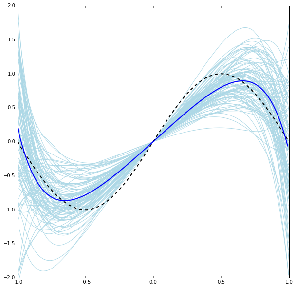
The regularization resulted in a much more well behaved spread around the mean than the unregulraized version. Although the regularization introduced an increase in bias, the decrease in variance was greater, which makes the overall risk smaller (with software help we can get numerical estimates for these values and see these changes for ourselves).

We can also examine the effect of regularization on the risk in light of our generalization bound. The following plot shows the contours of the squared difference loss of a linear model (two parameters). The red circle depicts our L2-regularization constraint $w_0^2 + w_1^2$.

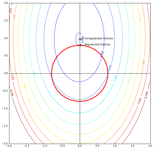
The plot shows that when the regularization is applied, the solution to the optimization problem shifted from its original position to the lowest value position that lies on the constraint circle. This means that for a solution to feasible, it has to be within that constraining circle. So you can think of the whole 2D grid as the hypothesis space before the regularization, and regularization comes to confine the hypothesis space into this red circle.

With this observation, we can think of the minimization problem:

as a direct translation of the generalization bound $R(h) \leq R_{\mathrm{emp}}(h) + C(|\mathcal{H}|)$, with the regularization term as a minimizer for the complexity term. The only piece missing from that translation is the definition of the loss function $L$. Here we used the squared difference, next time we’ll be looking into other loss functions and the underlying principle that combines them all.

References and Additional Readings

• Christopher M. Bishop. 2006. Pattern Recognition and Machine Learning (Information Science and Statistics). Springer-Verlag New York, Inc., Secaucus, NJ, USA.
• Abu-Mostafa, Y. S., Magdon-Ismail, M., & Lin, H. (2012). Learning from data: a short course.